Articles published in the magazine Astronomía |
December 2017
The two faces of August
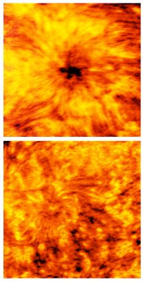
Solar activity divides the month of August into two clearly differentiated parts. A spot traveled through the disk alone and monopolized all the attention during the first half. It was the residual spot of group 12665 to which we referred last month. Almost did not undergo changes during those days, reducing its area only about 50 millionths of hemisphere, and for now, nothing presaged the important role it would acquire in the next rotation.
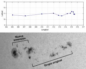
Two groups occupied the solar disk during the second half of the month. The most interesting was the first of them (NOAA 12671). During the first days, its spot p moved at an enormous speed towards the West (more than 1000 km / h) traveling 7 heliographic degrees in only 3 days. Little by little, it would slow down until it almost stopped. In addition, shortly after emerging from the limb, a new flow emersion occurred near its spot f. The old spots and the new ones originated a train of spots that came to cover about 250,000 km long.
The second group appeared on the 20th, and although it also had a respectable size (more than 100,000 km), its evolution was more monotonous and had almost disappeared when it reached the West limb.
We will leave the groups that appeared at the end of the month for the next article, since they are part of the extraordinary wave of activity in September.
Above: Displacement of 12671p, averaging the measurements of 5 observers. Below: Aspect of the group on August 17.
November 2017
The great group of Julio
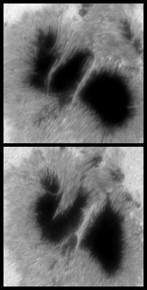
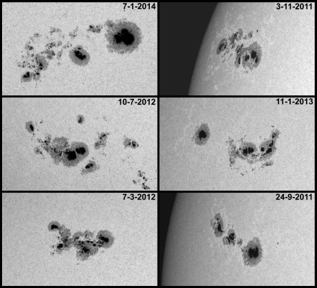
When due to its own movement, a spot is directed towards a larger and more stable one, its penumbras are generally joined and the nucleus loses speed, resulting in a spot with several umbras inside it. However, sometimes it is observed that the umbra maintains its movement, surrounding the main umbras, like a fluid circulating around an obstacle. Sometimes even, it can cause the rotation of the entire structure of the spot.
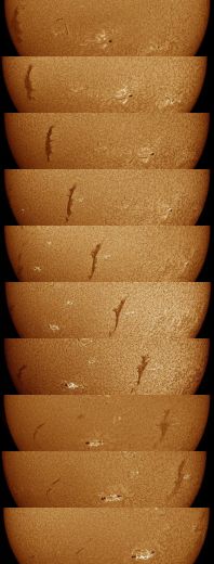
This process took place in region 12665, which appeared in limb on July 5. On the 7th there was an emersion in its central zone, and the coalescence of the new spot with the old one quickly took place. In principle, it seemed that the only effect would be the increase in size of the spot, which began to be detected with the naked eye since day 8. However, the most recent umbra slid to the south of the original, and once it was over, it turned north. In fact, the whole spot adopted an anti-clockwise rotation and both the striae of the penumbra, and the fibrils visible in Ha, showed a spiral arrangement, like a vortex.
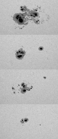
The images correspond to four days of transit, and the two main umbras have been indicated: A the oldest, and B the most recent. Although some days it was difficult to detect the umbras separately, given their proximity, the animations clearly show the development of the whole process.
The 12665 region will once again be the protagonist of two rotations with one of the most extraordinary groups we have seen in recent years. In fact, this was the first chapter of a remarkable outbreak of activity that has been developing since July, and we will comment on successive articles.
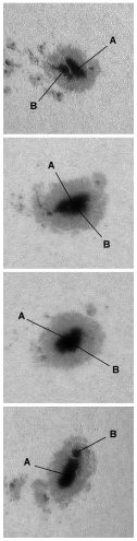
The main spot in the region 12665.
October 2017
The region 12645
We have repeatedly referred to magnetic field emersions that take place within the boundaries of a group or in its vicinity. A single isolated emersion will produce a group of simple morphology and generally not very active. However, the appearance of magnetic field often occurs discontinuously and depending on where and when the successive emersions occur, can lead to very active and complex formations. Actually, this is a circumstance that usually goes unnoticed, but which is of crucial importance when it comes to understanding the evolution of an active region.
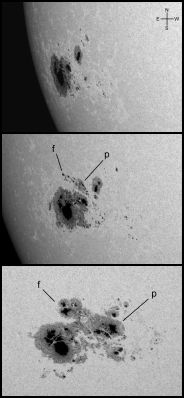
The group that developed in the region 12645 at the end of March, is a good example of several emersions that occur almost at the same point. The group appeared on the morning of the 27th near the eastern limbo. One after another, during the first days we witnessed a succession of bipolar emersions in the central part of the active region, and from March 2, once these ceased, the decline of the group began.
As the emersions grew, the spots separated and the result was a group with several spots of polarity p gathered in its western zone, and several of polarity f in the eastern zone. Some of the spots joined their penumbras giving rise to much larger spots, although keeping the umbras separated.
At the time of maximum development the group reached about 150,000 km and an area of some 900 millionth of hemisphere, reaching to be detected with the naked eye in the first days of April.
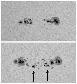
The 12645 region before and after one of the main bipolar emersions that took place in the center of the group.
September 2017
The region 12644
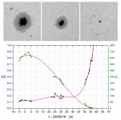
Although we are entering the minimum phase, it is still possible to observe groups of great interest. Such was the case of the one that occupied the 12644 region. It appeared on March 25, near the eastern limb and evolved rapidly, so that in only three days it reached its maximum development, at least in this first phase. At those times he showed only two good-sized spots occupying the p and f regions.
However, on April 1, a new emersion of flow began NW of the main spot. In the image it can be seen how the whole area had been altered a day later. The flares that occurred when the opposite polarities were found released much of the accumulated energy and the old p spot quickly disappeared. Despite being close to the limb, the images seem to corroborate that only the p spot of the new emersion persisted.
The region reappeared on April 17 with a spot (predictably, the same p that was hidden 15 days before), which was in the process of splitting. Perhaps the most interesting aspect during this transit was the movement of left-handed rotation that showed the set of both fragments (about 4º per day).
Only the main spot, already greatly diminished, would reach the west limb. However, he would still have the strength to maintain one more rotation. It reappeared on May 15 and this time offered a small nucleus surrounded by penumbra only in some sectors. It remained surprisingly stable, with hardly any size reduction, until day 22, when it began to dissipate rapidly.
The 12644 region during the three rotations that was visible.
July 2017
Days without spots
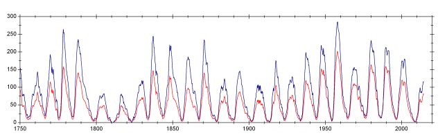
When Schwabe discovered the solar cycle, he produced a table where, for each year, he indicated the number of groups and the number of days without spots. In it it was clearly seen how both varied in antiphase, that is, when one increased the other decreased, and vice versa.
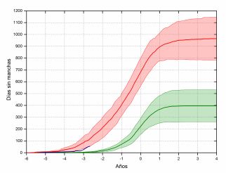
The number of days without spots in a given period can be used as an activity index. Schwabe used years, but nowadays it is more usual to use the monthly values, and to check its evolution the accumulated value is calculated. The total number of days without spots can vary greatly from one cycle to another. While the minimum of cycle 19 remained at 227, the last minimum reached the value of 817, and others have exceeded 1000.
Representing the cumulative number of days without spots as a function of time, and taking as reference the instant of the minimum, two types of cycles appear. In the graph, the lines indicate the average number of days without spots for both types, and the color bands are the standard deviation. The first shows a significant increase between two years before and after the minimum, reaching an average value of about 400. The second, shows days without spots in a greater interval of time, and can reach a total value close to 1000.
Since the last maximum, in the current cycle a total of 55 days without spots have been counted until the end of April. Assuming that this cycle will last 11 years, we would be at the lower limit of the red band (blue line). However, there is nothing to indicate that the next minimum will take place at the end of 2019, so we will still have to wait a while to find out what kind of minimum we are in.
June 2017
Radial motion in prominences
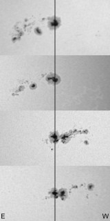
The images in white light are obtained in the area of the continuous spectrum, and the appearance of the Sun when we tune the Ha line is well known. However, moving only a little from the center of the line, without reaching the regions of the continuum, the chromosphere begins to be transparent showing the structures of the photosphere and phenomena hardly observed by amateurs, such as Ellerman's Bombs.
The prominences constitute a particular case. Although much of the prominence weakens to disappear when we leave the center of the line, however some areas are still visible and even increase in intensity. These zones may be different depending on whether we move to one or the other side of the line.
This behavior is due to the Doppler effect. If a part of the material moves towards the observer, its light will be shifted towards the blue and it will look better on that side of the center of the line. The opposite occurs if the material moves away from the observer.
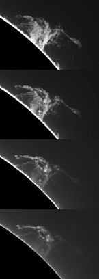
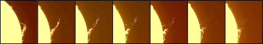
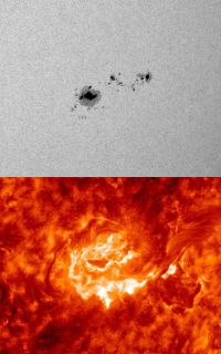
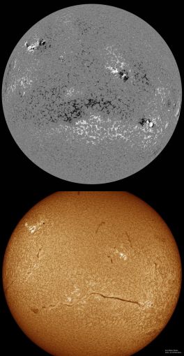
The black and white images show, from top to bottom, how the appearance of a prominence changes as we move from the center of the line to the blue. On the other hand, a very graphic way of showing movement along the visual is to obtain three images, one in the center and one on each side of the line. With them you can create a color image where blue indicates the material that approaches the observer, and red, which moves away.

May 2017
The cycle at the end of 2016
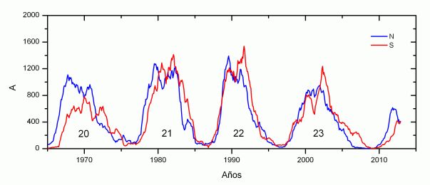
In 2016, the fall in activity continued, on the path to an increasingly closer minimum. Perhaps it is because the second maximum of the cycle was more intense, but the impression is that this descent is being quite fast, with a softened Wolf number that is already around 20 units. As for the total area, its monthly average has fallen almost 500 units in about six months, and if the trend is not corrected, we would find a zero area in a few weeks. All this points to a close minimum, but we must not forget that we only have about 8 years of cycle. If it meets the average, we would still have at least three long years with very little activity.
Possibly the most interesting at this time is the behavior of both hemispheres. Since 2013, activity in the North has remained almost constant and only at the end of 2016 has it shown signs of weakening. On the contrary, activity in the south has plummeted since the 2014 peak and is already at very low levels. Right now, almost all groups of spots appear in the north.
It is well known that the cycle in both hemispheres shows a lag so that one reaches the maximum before the other, and that lag is reversed every four or five cycles. For example, in the last five cycles, the north has advanced by reaching the maximum before, while the south has dominated the descending branch. This means that reversal should occur in this cycle. The fact is that since June 2015 the north is the hemisphere that predominates and it does not seem that this situation will change soon. Of course, with the Sun we always have to wait, but probably we have attended the expected reversal, and the South will advance to the north in the next cycle.
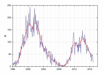
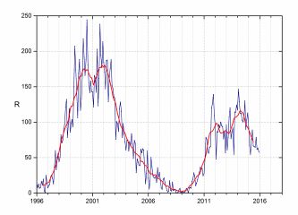
Monthly averages and smoothed values of Wolf's number in cycles 23 and 24.
April 2017
Polarities inverse ... .New cycle?
One of the groups that appeared in December was at 23º south latitude and had inverted polarities. A more recent group, from the beginning of February, also had an inverse polarity, although a somewhat lower latitude (15º north). This has raised the possibility that the new cycle has already begun and that these are its first manifestations.
In a new cycle, the groups have their polarities inverted with respect to the previous one and they are in middle latitudes. Now, the reciprocal is not true. It is estimated that approximately 3% of the groups have inverse polarities, and these can appear both at a maximum of activity, and at a minimum near the equator. Latitude is also not determinative because it depends on the evolution of Sporer's law and on the dispersion of group positions. It is not the same that a group appears at 20º of latitude at the minimum, than three years before.
The two-dimensional representation offered by the Maunder diagram may be the best way to separate the latitudes corresponding to each cycle. In the graph we can see the last groups of the previous cycle and the two wings corresponding to this cycle (Nº24). The red dots indicate the positions of the two groups mentioned above. It is evident that the group in the north belongs to the current cycle. The austral group may raise more doubts, but taking into account its proximity to the rest and that there is still travel to the next minimum (possibly about 2 or 3 years), it seems premature to include it in cycle 25.
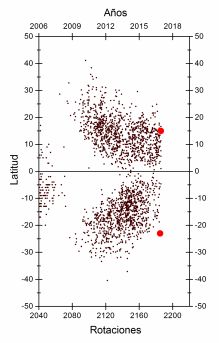
Maunder diagram with the positions of the two groups mentioned in the text.
March 2017
SOUL in the Sun
It is well known the impressive potential that ALMA has to reveal information about galaxies located in the limits of the Universe, or to dive into the depths of interstellar clouds to examine the birth of stars and planets, to give some examples. However, its ability to observe the Sun because its design prevents heat from damaging them, is not mentioned so often. In fact, it is the only facility in which the European Southern Observatory participates, trained to carry out this work.
The observatory can use two different and complementary techniques. A single antenna can make a quick sweep to get a low resolution image of the entire solar disk in a few minutes. The second option is to do interferometry using a few antennas separated by a certain distance. In this case, images of a small area of the disk are obtained with much more resolution.
Among other things, with these techniques you can examine the chromosphere giving a new perspective to the problem of warming the corona, or penetrate the structure of the prominences. You will also have the opportunity to examine an area of the little known solar spectrum, at wavelengths below 1mm.
The first observations have been released recently. The images were taken on December 18, 2015 and correspond to the main spot of the NOAA 12470 region. They are made at wavelengths of 1.25 and 3mm and basically show temperature differences at two different levels of the chromosphere (deeper to lower wavelength).
Images obtained with ALMA at wavelengths of 1.25 and 3mm.
February 2017
The activity in October
Despite the low solar activity that we are observing in these months, October offered us some interesting phenomena. At the end of September, a long filament was visible east of the meridian, with a length of half a million kilometers, that is, more than the distance between Earth and the Moon. Nothing else to begin October, day 1 of dawn, it erupted. Although other times these eruptions occur in response to a more or less close flare, this time it was not and it is difficult to know the cause. The CME (Coronal Mass Ejection) was fired towards the NE without reaching the Earth.
On day 2 a small group appeared near the east limb, and shortly afterwards there was a new magnetic field emersion slightly farther north. This developed much more and, in a certain way, came to engulf the first group. However, its activity in the form of flares was scarce, the most important being a B6.1 on October 4.
Day 3 emerged by limbo SE the most important spot of the month. With a surface of about 400 millionths of disk when crossing the meridian, it brushed the visibility with the naked eye. The penumbra contained several umbras and, while it was reduced in size, it was divided into two fragments that arrived already very diminished to west limb.
The rest of the month, the activity fell to quite low levels, more typical of the minimum that is getting closer.
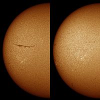
Images before and after the eruption of the filament commented on in the text. September 30 and October 1. (Courtesy: José Muñoz Reales)
January 2017
The great coronal hole of 2016
In the first months of 2015, a transequatorial coronal hole was developed, that is, it had an end at the north pole and after crossing the equator, it reached the middle latitudes of the southern hemisphere. The activity in the whole region that surrounded the great group that arose in June, left it reduced to the polar zone.
However, as of August 2015, it began to develop extraordinarily. By October 22, dominated much of the northern hemisphere pointing to Earth. Until mid-2016 it remained very intense, but with ups and downs in its dimensions, and issuing as pseudopods, up to three extensions that again crossed the equator to the south. The third, developed between June and August, did not disappear like the previous ones but was reinforced, so that at the end of October, the visible disk already occupied almost as much surface area as all the adjacent regions.
In a coronal hole the lines of magnetic field do not return to the surface but open to space, so that along them, the solar wind can flow freely. The stream of particles emanating from each of them will sweep the Solar System as the Sun rotates, and if the hole crosses the equator, as is the case, it can cause magnetic activity on our planet.
In past months we have witnessed geomagnetic storms every time the hole reached the solar meridian. We will see how it evolves in the future, but due to its characteristics, it has undoubtedly been one of the most outstanding solar phenomena of 2016.
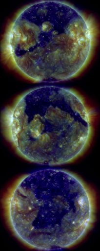
Three images of the coronal hole. From top to bottom: December 2015 and July and October 2016.
December 2016
Recovering Stereo
The Stereo mission consists of two ships (A and B) whose objective is to observe the Sun's hidden hemisphere and obtain three-dimensional views of different aspects of solar activity. A ship orbits at a speed somewhat greater than that of Earth, while the other moves a little more slowly. This movement leads them to stay behind the Sun for a while, and in those moments it is impossible to communicate with them. On October 1, 2014 communication with Stereo-B was lost while preparing to begin that transit.
The diagnostics suggest that after a reboot, one of the inertial systems began to send the wrong information, making the ship believe that it was spinning when in fact it was still. This caused that automatically, it tried to recover an orientation that already had, and the result was that it began to turn of uncontrolled way.
Each month, the NASA Deep Space Network made an attempt to reestablish communication and finally, on August 21, a weak signal was received indicating that the ship was still alive after almost two years. Although active, his condition is worrying. The fuel tanks are frozen, the battery is at 30% capacity, and the panels receive sunlight only at intervals.
NASA has already recovered other ships in similar situations. For example, SOHO had a similar problem in 1998, although in this case, it was only frozen for six weeks and was much closer to Earth. Let's hope that soon, the probe will be operational again and continue sending those data and images that help us understand our star a bit better.
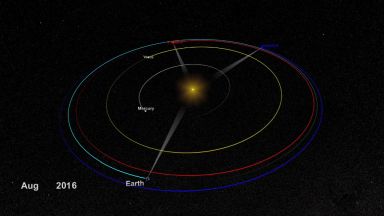
Stereo-A orbits (in red) and B (in blue).
November 2016
The NOAA 12565 - 12567 regions
Continuing with the series of large spots that have appeared in recent months, it is the turn of those who occupied the adjacent 12565 and 12567 regions. In fact, in July the highest and lowest values obtained this year were reached, at least so far . Several days without spots frame the biggest peak of the year, a little above that which took place in April.
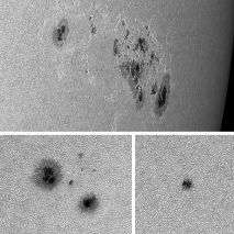
On the 11th, 12565 appeared in the eastern limb. It was a large spot with three main umbras inside. Throughout the days, its surface remained between 350 and 400 millionths of hemisphere, equivalent to four and a half times the surface of the Earth.
On July 14 and something further east, 12567 quickly emerged. In just a couple of days, its spot p was almost comparable to 12565, and with that size, both came to be seen with the naked eye in the vicinity of the center of the city. disk. To highlight the remarkable visible structures in the umbras, not only with bridges light but with a umbral granulation very appreciable.
During much of the transit there were only weak flares of class C. Near the west limb, the umbras were crossed by numerous light bridges and the penumbras became more irregular, beginning its decline. It was at that moment that the most important class M flares occurred.
In the next rotation, the zone contained several spots, but their positions, movements, and morphologies make it difficult to establish a connection between them and the July spots.
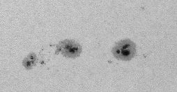
Image of NOAA 12565 - 12567 on July 18.
October 2016
The region NOAA 12546
After the great spot of April to which we dedicated the previous article, a new spot of large dimensions appeared in May, enduring no less than three rotations. At each transit, the spot received the numbers 12546, 12553, and 12562, respectively.
In the graph we have represented the variation of the area (in green) and that of the intensity (in blue) during the three transits. The intensity measurements are always affected by the stray light due to our atmosphere and the instruments. Therefore, we should not look at their absolute values, but rather at their relative variation.
The area almost reached 700 millionths of a hemisphere shortly after the first pass along the meridian, allowing observation with the naked eye. In June it was also appreciated by the naked eye, although its surface area had been reduced by half. In the last transit was already very small, but managed to stay until July 16.
The intensity correlates with the temperature and intensity of the magnetic field, so that at higher intensity, higher temperature and lower magnetic field. The graph shows the habitual behavior of other spots, keeping its intensity almost constant until a few days before its disappearance, moment in which it began to increase rapidly. What the graph reveals to us is how, as the magnetic field weakens, the spot shrinks in size and finally warms up to the temperature of the photosphere and disappears.
Images of NOAA 12546 on May 20, June 18 and July 12, with its variation in area and intensity.
September 2016
The NOAA 12529 region
Of the solar activity of the last months there are two facts that deserve to stand out: the first days without spots from the maximum past; and the presence of some huge spots that have recurred during several rotations. The largest was the denominated 12529, and 12542 in its second transit.
The spot emerged from the east on April 7, and soon after it was visible to the naked eye reaching an area equivalent to almost 6 times that of our planet. Its diameter reached about 60000 km (about 5 times the Earth). There are larger groups, but it is not often that a single isolated spot, with a regular shape, reaches those dimensions.
Despite its size, it had no major flares; only one of class M on day 18, which is due to having a single polarity almost monolithic. It only had a small intrusion of opposite polarity coinciding with the luminous bridge that is observed in the images.
The spot reappeared on May 4, greatly diminished and divided into two fragments that merged shortly after. By the time he reached the west limb, he was about to disappear. During its life, it was moving towards the west following a sinuous trajectory at an average speed of about 200 km / h. In the graph the positions are represented during both transits taking as reference the first measurement. The blue line is an adjustment curve where the points represent the positions at 12h UT between April 8 and May 15.
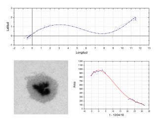
Image obtained on April 13 and two graphs showing the movement itself and the variation of the area.
July 2016
The mystery of the lost cycle (III)
The existence of a possible lost cycle at the end of the 18th century has recently received new evidence from the 10Be isotope analysis. The cosmic rays coming from our galaxy are responsible for generating this isotope in the atmosphere, and little by little it is deposited on the surface. By drilling in the ice of the polar areas, the different strata can be analyzed and the number of cosmic rays varied.
The interesting thing is that the amount of cosmic rays that reach the Earth depends on the interplanetary magnetic field and its polarity, which in turn depend on solar activity. In particular, the polarity is different in odd and even cycles, and can cause cosmic rays to increase just after a solar maximum or with a certain delay that can be up to about two years. Therefore, the amount of 10Be in the atmosphere can be used as an indirect measure of solar activity and give us clues as to whether we are in an even or odd cycle. That way, we could have an idea about whether the numbering of the previous cycles to # 5 is correct or not.
Although without discarding other hypotheses, the new analyzes carried out by a group of researchers from the University of Aarhus (Denmark), on ice cores collected in Greenland, suggest that the existence of a lost cycle is highly probable. However, unless new observations of that time appear, it is possible that we will never know with certainty if we have to add a new cycle to the solar activity of the last 400 years.
Ice core where the deposited layers are appreciated annually.
June 2016
The mystery of the lost cycle (II)
In 1870, the mathematician Elías Loomis, analyzing auroral observations and comparing them with the number of spots and the variation in magnetic declination, suggested that cycle number 4 was actually constituted by two short cycles of about 9 and 7 years. At that time, the idea was not accepted and was lethargic for more than a century.
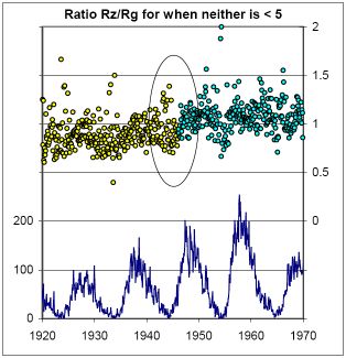
In 2001, the researchers Usoskin, Mursula and Kovaltsov rekindled it with the accumulated experience in all that time. It is easier to determine the number of groups than Wolf's number, so it may be more appropriate to reconstruct the activity from old observations. In the graph we have represented the number of groups during cycles 4 and 5. The data between the end of 1791 and the middle of 1793 are isolated observations that surely do not represent the group average. If we ignore them, the graph suggests the existence of a small cycle between 1793 and 1800.
Based on drawings by Staudacher and James Archibald Hamilton made during those years, the approximate latitudes of the registered groups have been measured. We know that at the beginning of a cycle the spots appear in mid-latitudes and approach the equator as the cycle progresses. What the positions of Staudacher and Hamilton show in the years 1793-1796 is not the typical activity of the decline of a cycle, but on the contrary, the groups appear in latitudes around 20º, far from the equator and more typical of the beginnings of a cycle.
However, there are also divergent opinions. The northern and southern hemispheres are rarely synchronized during the development of a cycle. In 2007, Zolotova and Ponyavin suggested that the duration of cycle 4 was due to an exceptionally high lag between activity in both hemispheres.
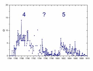
Monthly averages of the number of groups during cycles 4 and 5.
May 2016
The mystery of the lost cycle (I)
It is often considered that Wolf's series of numbers is quite homogeneous, but it contains a small (or large) mystery that may never be solved.
When Wolf developed the number that bears his name he tried to reconstruct the previous cycles. However, there was a major difficulty and that is that the available data was not continuous. To give an example, in the years 1792 and 1793 there are only 20 observations that cover 16 days, and 12 of them correspond to 8 consecutive days.
To cover the gaps, Wolf decided to interpolate using the diurnal variation of the magnetic declination as a reference. A magnetic needle deviates to the east and west at the end of the day, and the magnitude of that deviation correlates quite well with Wolf's number, so it can be used as a calibration method. The point is that the Wolf numbers prior to 1847 are a mixture of observed and interpolated data. This can be seen particularly in cycle # 4, which took place just before the Dalton minimum, a succession of very little active cycles.
Actually, cycle # 4 seems a bit special. On the one hand, it is the longest known cycle spanning 163 months; October 1784 to April 1798. Also violates the rule of Gnevyshev-Ohl, a general principle that tells us that an odd cycle, usually has more activity than the previous cycle.
However, the Gnevyshev-Ohl rule has seen other exceptions, and some cycle has to be the longest, so is it as special as it seems, or is it a normal cycle? To be continue…
The cycle nº4.
April 2016
How is the cycle going?
The maximum activity, is already behind and at this time we find some values of the number of Wolf that are approximately half of those that were reached in 2014. Less and less prominent groups are the main characteristic of this phase, although from time to time as long as they appear spots with enough size to be seen with the naked eye. Without going any further, December offered us a magnificent specimen that appreciated without optical aid during a large part of its transit.
Activity by hemispheres is even more interesting. The north-south asymmetry seems to have a periodic behavior, so that every 4 or 5 cycles is reversed. The northern hemisphere peaked at the end of 2011, and after an initial drop, it has remained constant for about 2 years. The maximum of 2014 corresponds to the southern hemisphere, and this is the fifth consecutive cycle in which the north advances to the south.
However, the decline in austral activity has been so pronounced that since the middle of 2015, the north has become predominant. Of course, little time has passed and it remains to be seen if it is a random investment and the previous trend will recover, or else it will be maintained, and during the next cycle, the south will go ahead.
Making forecasts at this point is almost impossible. However, the forecast of the Belgian Observatory suggests Wolf numbers smoothed between 25 and 50 (depending on the model) for one year; and extrapolating the slope, we would have to wait for the next minimum not before 2019.
Graph of cycles 23 and 24, updated to December 2015.
March 2016
November
November started with an interesting group, followed with an interesting filament, and ended with little interest.
The group was in the region NOAA12443 and had two well-developed spots, while in its f region there were many smaller spots. When in the region p of a group there are two or more predominant spots, they are generally the consequence of different emersions, which in this case, should have occurred in the occult hemisphere, since in the previous rotation there were no spots in that region. The group reached about 200,000 km long and dissipated somewhat quickly once the meridian had passed. During its transit it produced some 70 flares, although only two reached the M classification.
On November 6 began to emerge through limbo E, a filament, which was the most interesting mid-month. Usually, a filament of that length separates large unipolar areas and has a more or less rectilinear shape. In this case, it had an almost circular shape (although it lacked the eastern sector), because it delimited a kind of island of polarity p surrounded by areas of polarity f.
On day 15, the filament erupted at its southern end, although its northern part fell back to the surface. The photographs of José Muñoz show the before and after the eruption.
Except for some other prominence, November ended with very little activity, with small groups and short life, which presage a minimum closer and closer.
El 6 de Noviembre empezó a asomar por el limbo E, un filamento, que fue lo más interesante de mediados de mes. Habitualmente, un filamento de esa longitud separa grandes zonas unipolares y tiene una forma más o menos rectilínea. En este caso, poseía una forma casi circular (aunque le faltaba el sector oriental), debido a que delimitaba una especie de isla de polaridad p rodeada de zonas de polaridad f.
El día 15, el filamento entro en erupción por su extremo austral, aunque su parte norte volvía a caer sobre la superficie. Las fotografías de José Muñoz muestran el antes y después de la erupción.
Salvo alguna que otra protuberancia, Noviembre finalizó con muy poca actividad, con grupos pequeños y de corta vida, que presagian un mínimo cada vez más cercano.
Images of days 15 and 16, before and after the eruption of the austral filament (Courtesy José Muñoz)
February 2016
Happy Birthday
On December 2, it was 20 years since the launch of the SOHO (Solar and Heliospheric Observatory).
The ship, fruit of ESA - NASA collaboration, is orbiting around the Lagrange point L1, which guarantees an uninterrupted view of the Sun. In all this time it has managed to observe almost two complete solar cycles, with one exception, in 1998, when contact with her was lost for several months.
SOHO can obtain images through four wavelengths of extreme ultraviolet (the first systematic from space), two coronagraphs, and in the continuum, in addition to making magnetograms. Due to the quantity, quality and variety of the images, it has only been surpassed by the SDO, although the latter does not have coronagraphs.
The use of coronagraphs is of special interest given that their situation, on the Sun - Earth line, allows them to detect those eruptions that will later reach the Earth (more than 20,000 in these years). Also, thanks to them you can observe comets, having discovered more than any other observer or observatory.
In addition to the images, SOHO is able to analyze particles and isotopes, measure solar radiation or perform heliosismography, for example. All the observations collected in these years are undoubtedly one of the most complete databases that currently exist on solar activity.

January 2016
A filament and a group
We spoke recently of the formation and eruption of filaments, and precisely, September offered us the opportunity to observe the evolution of a magnificent filament. It began to appear in the limb on the 15th, and during its transit we had the chance to observe it from different angles. This circumstance allowed us to check its three-dimensional structure, as can be seen in the magnificent sequence by José Muñoz.
A filament usually has the form of a vertical sheet, suspended in the neutral line between both magnetic polarities. That is why it was much thinner in the meridian (when we saw the sheet of singing), which in the vicinity of the limb (when we saw it sideways).
In last days it was increasing in size, erupting on the 30th in the morning, just when it was in limb.
The second protagonist of the month was the region 12422, which developed further to the E. of the filament. It appeared on the 22nd and evolved rapidly, reaching almost 150,000 km in length.
The polarities were mixed in their central zone and in some points a certain delta configuration was originated (both polarities in the same penumbra). In these circumstances it is easy to jump the spark, and from day 26 there were multiple flares of type M. As a result, the region was losing intensity and disappeared after the limb already in frank decline.
Sequence obtained by José Muñoz between September 19 and 28, showing the filament and the region 12422
December 2015
The two groups of August
A look at the August graphs shows much more pronounced variations in the area than in Wolf's number, which is usually indicative of few groups, but large. In effect, two groups stand out over the rest during this month, to the point that they became visible to the naked eye.
The first (12396) appeared on day 3, and although it had a rapid development, little else is possible except for the enormous size reached by its spot p. It produced more than 30 flares, but all of type C, and it was hidden by limbo W on day 14 already in full decline.
The second (12403) was much more entertaining. It appeared in the limbo on the 18th, and shortly afterwards there were two emersions of flow, one to the north and one to the south, which altered the entire region. On day 20, for example, it presented a morphology that was difficult to classify according to the types of use.
Of both emersions, the southern one predominated, and it extended quite a lot in time. At least, until the 25th we were able to observe the formation of spots in the central zone and its rapid movement towards the ends of the group. Precisely in its central zone there was quite a mixture of polarities, which translated into more than 120 flares, 18 of which were of type M.
The group hid behind the limb on the 30th, although its spot would manage to keep at least two more rotations.
Finally, it is worth mentioning that this group appeared in a complex of activity in the southern hemisphere, which has been offering groups almost continuously since March.
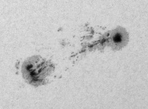
Image of NOAA 12403 obtained on August 24.
November 2015
Prominences
The idea that prominences are explosions; and even that its eruptions are always related to explosive phenomena, it is very widespread. Certainly, some originate as a result of flares, but most tend to be durable formations, which can be maintained during several rotations.
A prominences or filament is always formed in the neutral line that separates both magnetic polarities. In general, its formation begins when the spicules begin to line up parallel to the neutral line, revealing a kind of "channel" inside which begins to condense colder and denser material, in a process that can last several days.
Once formed, the filament can reach enormous lengths, and then it can become destabilized. The cause may be the shock wave of a distant flare or simply, changes in the magnetic fields near the neutral line.
When that happens, the filament begins to ascend, sometimes through the center, or at one end. As it goes up, it accelerates, and ends up being fired into space. This process hardly affects the "channel", so that material can continue condensing inside. In fact, it is relatively frequent, that after an eruption, we see a new filament forming in the same position as the previous one.
In recent months we have observed some beautiful eruptions of this type; and serve as sample the sequence recorded by José Rosell on June 3.
October 2015
The Waldmeier effect
Among the modifications introduced by Wolf's new official number series, one of the most important is the correction of the "Waldmeier effect".
In 1945, Waldmeier is appointed director of the Zurich Observatory, and continues to obtain Wolf's series of numbers, but modifies the counting method used until then.
For Wolf, each spot was worth a unit, although he only counted the largest to avoid the effects of seeing. Their successors counted all the spots, so that their values were 67% higher (a factor of 0.6 was introduced to match both methods), but each spot was still worth one unit.
For Waldmeier, however, a spot could be between 1 and 5, depending on its size. Unlike in the previous case, it did not introduce any correction factor, so Wolf's numbers were overestimated after 1945.
To complete those cloudy days in Zurich, Waldmeier used data from a secondary station in Locarno (Switzerland), and instructed them on their counting method. When in 1981, the SIDC took charge of maintaining Wolf's series of numbers, it used Locarno as a reference station, and thus, the inconsistency originated by Waldmeier, has remained to this day.
In recent years, Locarno has been obtaining 2 parallel series with both methods; and from the comparison it is deduced that the method employed since 1945 increases the values by 17%. After the correction made this year, Locarno remains as a reference station, but definitively discarding the Waldmeier method.
Comparing Wolf's number with the number of groups, a leap in the graph is clearly visible, revealing a different counting method.
September 2015
New series of Wolf numbers
For Wolf's number, on July 1 will mark a before and after. For more than 100 years, the series had not undergone any revision; and over time, had accumulated certain inconsistencies that needed to be reviewed and corrected. To that end, a team of scientists has met in recent years in four "SSN-Workshops", and finally, the result of their work has come to light on July 1, with the publication of a new series.
Wolf's successor, Alfred Wolfer, modified the counting method used by the first, and it soon became apparent that in order to match Wolfer's data with Wolf's, it was necessary to multiply it by 0.6. Since then it has been doing so with the entire series to keep as a reference to Wolf.
Perhaps the most striking modification in the new series is the elimination of this factor. Now, Wolf's values fit the series, instead of adjusting the entire series to Wolf's data. This translates into a change of scale, increasing the values by 67%.
Another correction of more draft, is the suppression of the "Waldmeier effect". From 1945, Waldmeier began to assign a weight to the spots, so that they could be different depending on their size or position on the disc. The Locarno Observatory, the SIDC reference station, continued to use this method, with which values are obtained that are 17% higher than with the traditional method.
The new series corrects the values since 1945 and retrieves the Wolfer method, which is used by almost all stations.
Other modifications affect the discrepancy with the F10.7 index observed in recent years, and with the number of groups before 1880. Of course, there is still much work ahead to verify the impact that this new series will have on our knowledge of the Sun.
Comparison between the old series of Wolf numbers (red), and the new one (blue)
July - August 2015
The storm of March
Although magnetic storms are generally associated with a greater number of spots or with powerful flares, this is not always the case.
In mid-March there was hardly anything noteworthy about the record, except for one region (12297) of medium size. When it emerged from limb it was only a residual spot, but soon a new bipolar group appeared, whose spot f collided with the original. During the whole process, the region produced around 150 flares, one of them class X on day 11, but none of them seriously affected our planet, ... except one.
On the 15th, when the region was already heading towards the west, there was a C9.1 flare, that is, nothing extraordinary. Two days later, the ACE probe was the first to register the shock wave, moving at about 700 km/sec. The interesting thing is that the magnetic field that dragged the shock wave was very negative, oriented in the opposite direction to that of our planet. In those circumstances, our defenses are weakened and the storm is triggered.
The intensity of a storm is quantified with the Kp index, which is an average of the magnetic disturbances recorded in several stations spread across the planet, in 3h intervals. Kp varies from 0 to 9.
During the afternoon of the 17th, Kp reached the value 8, becoming the most intense storm of this cycle. In fact, we must go back 10 years (until May 15, 2005) to find another stronger storm, although still, it stayed away from historical storms like 1989 or 2003.
Auroras were recorded from France or Germany, but they did not reach our latitudes, for which a maximum value of Kp would have been required. Maybe the next one ...
Images of region 12297 at the time of the March 15 flare (SDO)
June 2015
The filament of February
When a group of spots appears, a filament usually forms at the location of the neutral line. This is a characteristic of every filament or prominence, that is to say, to situate itself in the border that separates both polarities.
In these early phases, usually the filament does not have a large extension, because the magnetic fields are concentrated in the region of the group. However, when the group of spots disappears, the fields disperse on the surface, becoming part of large unipolar sectors. In fact, if we go around the solar circumference at medium latitudes, we often find a succession of sectors with alternative polarities p and f.
The neutral line separating these sectors can reach a large extent, and consequently, when occupied by a filament, it can also develop enormously.
The previous process occurred in the austral activity complex to which we have referred in recent months. In February, when it had stopped producing spots and its magnetic fields had already dispersed towards the pole, it offered us a gigantic filament, more than a million kilometers long. It was so long, that it took almost a week to emerge through limbo and see himself completely; and while one end had just appeared in the east, the other was already approaching the west limb.
In the photo of José Muñoz, obtained on February 10, its extension can be seen, and the magnetogram of the SDO helps to see its situation, separating the polarities of the complex.
In March and April only several sections were seen, each time smaller, although the "channel" where it had been formed, could still be clearly seen in the chromosphere.
Magnetogram of SDO and image in H-alpha obtained by José Muñoz on February 10th.
May 2015
The decline of an complex of activity
The complex of activity where the great group of October appeared, continued to be the protagonist in the following months. It may not be coincidence that the sharp decline in general activity experienced in February coincided with the time when this region stopped producing sunspots groups.
During the November transit, the two main October spots were maintained, although they were already diminished in size. The flares continued to be numerous but more moderate in intensity, not exceeding in any case, the classification C. The group quickly lost strength as it approached the west limb, announcing an early disappearance.
What appeared in the east in December, were only a few small spots (perhaps the last rest of 12192), but on the 12th a new group began to form, which in continuous impulses adopted a quite complex magnetic configuration.
Two emersions of flow at a short distance, led to find the spot p of one of them, with the f of the other, and the consequence was immediate: about a hundred flares throughout the transit. Most were type C, but some M, and above all, an X on day 20.
By not knowing what happened in the occult hemisphere, it is not clear if the spots that were seen during the January transit were the same as in the previous one or corresponded to a new group. In any case, their positions were very similar, although their level of activity had decreased considerably (fifteen flares, all of type C).
The complex has not returned to produce spots. In February he offered us a bright facular region, but already very extensive and disseminated. In Ha, however, the show was maintained thanks to a giant filament, which will be the protagonist of our next article.
Groups of spots produced by the activity complex, from October to January. (Images of the SDO)
April 2015
Light bridges
The region 12192, which we saw in October, serves as a pretext to talk about the light bridges, given that he gave us some magnificent examples of them.
A bright bridge is a bright structure that crosses the umbra of a spot. They are usually elongated and have one or both ends connected to the penumbra or other bridges, although in rare cases they may appear isolated inside the umbra (a very striking case occurred in region 12109, on July 11).
In general, they tend to be more frequent during the formation of a spot, when the coalescence of other smaller spots occurs, or, in the fragmentation prior to their disappearance, but this does not mean that they can not be present for almost the entire life of the spot
Being surrounded by the darkness of the umbra, sometimes by contrast, they can appear to be very luminous, but usually they do not reach the brightness of the photosphere.
Morphologically, they can be classified into two types: those that divide two or more nuclei (usually the brightest), or those that appear as a penetration of material into a nucleus. They can also be classified according to their structure: some are grainy, and others appear to be made up of filaments, as an extension of the penumbra structure.
The generalized opinion is that solar convection opens from below, through the powerful magnetic field that forms the spot, reaching the surface. However, despite being easily observable, only its basic characteristics are known, and there are still many unknowns about its formation and properties.
Keeping track of its birth and evolution is undoubtedly a fascinating subject of observation available to almost any telescope.
Light bridges in the region 12192, on October 25 and 26 (Courtesy of the authors).
March 2015
The region 12192 (2)
The appearance of region 12192 in October made us wonder whether it really was as exceptional as it seemed. Of course, everything depends on the feature we choose. Here we will look at the surface reached and the flares produced.
Area data, in millionths of hemisphere, are valid since 1874 (Greenwich / NOAA). The 15 largest groups have been included in the table since then.
The eldest, with difference is the one that appeared in March 1947; and we still remember the huge groups of cycle 22, four of which are listed. As a curious fact, the "ranking" is dominated by cycles 18 and 22, as if some cycles were more likely to produce gigantic groups.
| Nº | Fecha | Grupo | Area | Ciclo |
| 1 | Marzo1947 | 1488603 | 6132 | 18 |
| 2 | Enero 1946 | 1441702 | 5202 | 18 |
| 3 | Marzo1989 | 05395 | 5040 | 22 |
| 4 | Mayo1951 | 1676304 | 4865 | 18 |
| 5 | Julio 1946 | 1458503 | 4720 | 18 |
| 6 | Marzo 1947 | 1485104 | 4554 | 18 |
| 7 | Junio 1982 | 03776 | 4340 | 21 |
| 8 | Agosto 1989 | 05669 | 4312 | 22 |
| 9 | Noviembre 1990 | 06368 | 4312 | 22 |
| 10 | Junio 1988 | 05060 | 4060 | 22 |
| 11 | Julio 1982 | 03804 | 4018 | 21 |
| 12 | Octubre 2014 | 12192 | 3850 | 24 |
| 13 | Enero 1926 | 986103 | 3716 | 16 |
| 14 | Febrero 1982 | 03594 | 3696 | 21 |
| 15 | Octubre 2003 | 10486 | 3654 | 23 |
And the group 12192? As it occupies the position No. 12, slightly ahead of October 2003. In fact, we must go back 24 years to find a larger group.
Regarding the flares, the region produced 6 class X. There are systematic data since 1976 and since then, there have only been 8 groups that have produced 6 X flares, and another 5 have exceeded that figure. However, the most powerful flare occurred in 12192, was an X3; far from the October 28, 2003, or the March 15, 1989.
Despite this last fact, there is no doubt that we are facing an exceptional group, and that it will probably be several years before seeing another similar one. I wish we were wrong !.
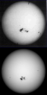
Imagen del grupo de Marzo de 1947 (arriba) comparado con 12192 (abajo).
February 2015
The region 12192
When large groups appear, such as that of region 12192, the observation is interesting because they are unusual phenomena, but if we also ask about their origin and evolution, we are facing very dynamic processes of solar activity, which help interpret other more frequent cases.
The large spot that appeared on October 16 had almost the same position as 12172, a residual spot from the previous rotation. What happened in the occult hemisphere? It is difficult to say, but probably the appearance of new spots further west, reactivated the whole area, so that when it reappeared in limbo, it already had an area equivalent to that of 15 planets like Earth.
It was the 19th when a phenomenon occurred that would mark its subsequent evolution. The magnetic field does not appear on the surface continuously but in impulses, and one of them occurred just north of the group, in the form of emersion of bipolar flow. In the image we have indicated the spots p and f corresponding to said emersion.
The axis of the group was directed in the NW-SE direction, but the one of the new emersion was located in the SW-NE direction, so that when it was developed, the new p-spot was embedded in the original group (as if we had two groups intertwined ). If the area was already large, now it continued to increase until day 23, when it almost doubled (similar to about 27 planets like Earth).
The successive flares relaxed the magnetic configuration of the group, and from day 23 the spots began to disappear. However, the two main ones still had sufficient intensity to withstand a couple of more rotations, remaining visible at least during the transits of November and December.
Images obtained by the SDO corresponding to days 18, 19 and 23 of October.
January 2015
Proper motions
For several years we have measured the position of sunspots. We usually focus on the main ones, p and f (western and eastern, respectively). The measurements taken daily show small changes that show that they move on the solar disk.
However there are some effects to be taken into account, one due to the differential rotation of the Sun on its axis and another to the translation of the Earth around the Sun.
Since the sun is gaseous, its period of rotation is not uniform as that of a solid, it rotates more rapidly at the equator and decreases with latitude towards the poles. For that reason, spots located at different latitudes can be ahead or delayed with respect to the network of coordinates. Apparently, a spot at high latitude will appear to move eastward; and to the west if it is close to the equator.
On the other hand, the fact of being placed on a moving object like the Earth, makes appear another apparent displacement
Once these effects are eliminated, there is still a continuous variation throughout the days. We derive this drift as the actual movement of the spot and hence the label we have given them of "proper motions" (not apparent).
These measures, on the other hand, allow us to obtain the rotation in that particular point and with it, calculate the period. On the other hand, we can make an estimate of the length traveled and its speed in km / h.
Motions of the 3 main spots of the 12056 region, between May 8 and 16, 2014. The coordinates are longitude and latitude, taking as reference the first measurement of one of the spots (1º = 12,000 km). The spots p and f were part of the same dipole, while the spot fn was the residue of a previous group.
December 2014
Review
In this month of December, it seems to be customary to make a small balance of what the previous months have been, so we will review what this 2014 has been as far as solar activity is concerned.
Within the context of the cycle, at the beginning of the year (February), we have the greatest increase in activity, which gives us the maximum values of Wolf's number, surpassing the highest numbers reached at the end of 2011. In that occasion was the northern hemisphere responsible for the rise, while in this year it has been the southern hemisphere. This has continued to dominate in this phase of the cycle that will culminate, as seen in the following months, after a break in mid-year, in a rebound that probably represents the peak of the current cycle to take the inflection path to a new minimum.
In short, the year that ends marks a point of maximum activity in February that has been relaxing until annual minimums in the month of June. From that point a new rise in activity, always with the southern hemisphere as the protagonist, marks a new maximum in September that exceeds even what was achieved in February.
Except surprises can not expect new peaks so high in the coming months, already started 2015.
In particular two active regions have marked the year, the first NOAA 11944 that was associated with the 11967 with a final outcome in 11990, was the protagonist in the first months.
In October an immense compact spot NOAA 12192 monopolized the attention throughout its development in the solar disk, being the largest observed since 2003. In coming months we will return to it to review its development.
November 2014
Is there a Livingston-Penn effect?
Although we address this issue at the beginning of the year, it is worth retaking it since it was dealt with in the IV SSN Workshop held in May in Locarno. Recall that, from measurements made since the late 90s, both researchers came to the conclusion that the magnetic field of the spots was decreasing, and consequently that the spots would disappear in a few years.
In a paper prepared by Fraser T. Watson, and Matthew J. Penn and William C. Livingston themselves, they note that their conclusions do not coincide with those obtained from other data sets, and recognize that the data obtained before 2006, they contain an observational bias.
To understand it, suppose we observe the Sun one day when it has spots. We may see large spots, or maybe not, but what we are almost always going to see are small spots with weak magnetic fields. However, in the Livingston-Penn data, these small spots are practically absent during the whole cycle 23, since there was a selection and only the largest ones were measured.
The consequence is double. The magnetic fields in cycle 24 are smaller because in this case small spots are included, and on the other hand, the decrease observed before 2009 is no more than a reflection of the decrease towards the minimum of cycle 23.
Of particular interest was also the intervention of Giuliana de Toma (High Altitude Observatory), where from a complete set of data obtained in the San Fernando Observatory, reproduced the Livingston-Penn effect, simply eliminating the small spots of cycle 23.
Therefore, there does not seem to be any evidence of changes in the intensity of the spots, or that they will soon disappear from the Sun.
October 2014
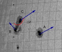
The region 12056
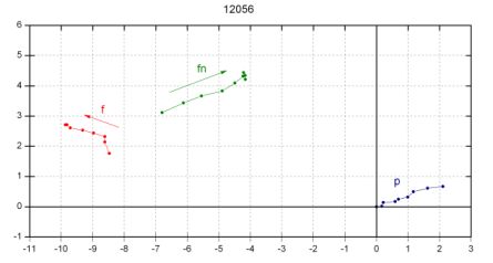
The movement of the spots is one of the main causes that produce flares. Two spots of opposite polarities can approach, or come into contact, and that closeness often causes the reconfiguration of the magnetic field and the release of the energy we know as flare.
A recent case that illustrates this process occurred in the region 12056. This region emerged in the main activity complex of the northern hemisphere, and appeared in limb on May 5. It showed 3 main spots, which in the figure we have named A, B and C. While A and C had polarity p, B had a polarity f.
Given the distribution of polarities, it can be assumed that C was the residual spot of an old group that evolved in the occult hemisphere, and that A and B constituted a bipolar group that emerged later to the southwest.
The position measurements show that A and C moved almost parallel to the northwest, while B moved to the northeast. These displacements approached spots B and C, joining their shadows and creating what is known as delta configuration.
In the image, the arrows indicate their movements and the red trace indicates approximately the neutral line that separated both polarities. It was along that line where the powerful flare (M5.2) of May 8 originated.
Subsequently, both spots were separated at a relative speed of about 250 km / h, while they were reduced in size and the magnetic configuration relaxed; producing from then on, only class C flares. The spots ended up disappearing a few days later, when the region was already close to the west limb.
September 2014
The region 11944 - 11967
In January we were able to witness the appearance of an activity complex that offered us the largest set of spots in the cycle. Its evolution was somewhat difficult to interpret given the changes that took place during its passage through the occult hemisphere.
In the image we have represented the aspect that presented the days 6 and 10 of January (1st transit), and 2 and 5 February (2nd transit). The images have been passed to rectangular projection, to eliminate the distortion by perspective, and we have horizontally centered the main spot, which was the only one that survived all that time, without taking into account, therefore, the proper motion.
When the region reappeared in limbo at the end of January, the situation was confused. It seemed that he had "turned around", since now the main spot was to the East.
Thanks to the Stereo ships, which can observe the hidden hemisphere from Earth, we have enough clues to understand what happened. On January 17 and 18 there is a strong increase in brightness west of the main spot, which can be associated with the appearance of a new group, and soon after, between days 21 and 22, it can be seen as "turn off" the area to the East.
Thus, it seems that all but the main spot disappeared in the hidden hemisphere, being replaced by new ones to the west.
During both months, this complex produced up to 6 main groups, and many others of small size, consisting mainly of pores.
July - August 2014
Activity complexes
When looking for cycles in Wolf's numbers, in addition to the more obvious one of 11 years, it is usual to find another one with a duration of approximately one month (similar to the solar rotation period). This period is not permanent, but usually occurs at intervals ranging from three months to more than a year, being absent at other times.
As it is uncommon for a group of spots to last more than three months, it seems logical to think that this period is due to a different form of activity, which persists for months in the same area and appears before us with each solar rotation.
A limited region of the solar surface is called an activity complex, which produces groups of spots for several months almost continuously. They can exceed 20º in length, and remain active for more than a year. However, let's not look for a precise definition. If we lack a definition of what a group is, even more than it is a complex.
In fact, it is very rare to find references in informative texts, and when we search for research articles, each author uses different definitions and methods, sometimes reaching inconsistent conclusions. It is, therefore, a little-known type of activity, despite being easy to observe.
In the current cycle, the complexes are being shown in line with the level of general activity, being less abundant and active than in previous cycles. The most durable so far, it appeared in the northern hemisphere and maintained its activity from January 2011 to April 2012.
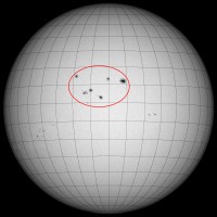
Image obtained on May 11 where a recent activity complex has been marked. This complex has accounted for approximately 40% of all groups that have appeared in the northern hemisphere since March, and has been largely responsible for the activity peaks of April and May.
June 2014
4th SSN Workshop
The fourth edition of the "SSN Workshop" was held in Locarno, Switzerland between May 19 and 23. These workshops, which began in 2011, present a great interest for all of us who are dedicated to observing the Sun, given that they have, among other objectives, to review Wolf's historical series of numbers, and provide the necessary tools to maintain it in the future. .
Wolf's number is probably the most extensive time series that exists in science, which makes it widely used, not only in solar physics, but in other areas, such as climatology, statistics or chaos theory ... However, It has certain inconsistencies that need to be understood and corrected.
Perhaps the most important is the one known as "Waldmeier discontinuity". Waldmeier, director of the Observatory of Zurich, modified the way to do the spot counts around 1946, and since then, the values obtained are overestimated with respect to the previous ones.
In addition, it is necessary to establish a stronger relationship between Wolf's number and other activity indices. So for example, there is another way to do the counting using only groups of spots; and although the activity derived from both indices coincides in many points, there is an important discrepancy before 1885.
The bases established in this meeting will lead to the publication in the near future of a new more complete and consistent series.
On the other hand, they have also analyzed various historical aspects, or some characteristics of solar activity in recent cycles. Of all this we will give account in future articles.

May 2014
The area measurements
During January and February, the Sun has offered us the most extensive set of spots we have in the cycle, while the total area reached the highest values since the last cycle.
The area is one of the most commonly used activity indices, along with the Wolf number and the flow at 10.7 cm. The most complete series of areas is that of the Greenwich Observatory, whose data span from 1874 to 1976 and were obtained on photographic plates. Since the Observatory ceased this activity, other observatories have tried to resume their work and an important effort has been made to adequately calibrate the series obtained by the different stations.
After Greenwich, the most complete series corresponds to the Debrecen Observatory (Hungary), which started its series in 1977, also using white light photographs.
In 1981, the Solar Optical Observing Network (SOON) began its activity, although with a different methodology. There are several similar telescopes located in different terrestrial lengths, and instead of photographs, they use drawings with a diameter of 18 cm. The measurements are made with a set of templates with circles and ellipses for the areas and others for the positions. SOON sacrifices accuracy for the sake of speed, trying to keep data collection almost in real time.
Although after months, Wolf number and area increase and decrease with solar activity, on a temporary scale of days they are not always synchronized. This is because both indices measure different things. The first is related to the number of spots, while the second tells us about its size.
So, they are complementary ways of measuring solar activity. Many small groups will increase Wolf's number, but not the area; and vice versa, a few large groups will increase the area, but keep Wolf's number at moderate levels.
April 2014
The Carrington event (III).- The storm
On September 2, 1859, the shockwave originated in the Sun 17h before arrived on our planet. In Kew and Greenwich stations recorded magnetic field oscillations that exceeded the top of the scale, which makes it difficult to quantify. In Bombay, on the contrary, the records were made by hand and show the highest fluctuations observed in a magnetic storm. However, the speed of the variation makes its interpretation difficult, and there is evidence that, in part, its origin is in the ionosphere, and therefore, it would not be a representative record.
The indexes that are used to measure the intensity of a storm were not used in 1859, so a direct comparison is not possible. However, estimates show that it was not significantly more intense than the largest storms observed since then.
The auroras of 1859 came to be seen at 20º latitude, which is not frequent. From 1849 to 1958 there are only 6 auroras well documented that have exceeded a latitude of 30º. However, the storm of 1872, whose aurora reached 19 º, occupies a modest place among the most intense recorded.
Perhaps the most spectacular effects took place on the telegraphic networks of the time. Some devices were disabled, and others could operate without batteries thanks to the currents induced in the cables. In some cases, these caused small fires.
The truth is that various studies show the special vulnerability of telegraph networks to the effects of a magnetic storm, and one wonders to what extent they can be extrapolated to current technology. Other comparable storms that occurred more recently (1989 or 2003, for example), did not have devastating effects. At most, there were blackouts, interference in communications, etc ... but after a few hours or days, the situation was normalized.
March 2014
The event Carrington (II).- The flare
The flares are classified using their emission in X-rays, and thus for example, X5 is equivalent to 5 x 10⁻⁴ W/m2. Now, how can we classify a flare that occurred in 1859, when the X-rays were not even known? We can only compare its characteristics with those of more recent ones and assume a high degree of uncertainty.
The radiation emitted usually causes a disturbance in our magnetic field, called SFE (Solar Flare Effect). Considering the intensity of the SFE, the flare of 1859 is the fourth in order of importance, being surpassed by others in 1942 and 2003
On the other hand, the time it took for the shockwave to reach Earth was only 17.6h, surpassed by the event of August 4, 1972, and similar to that of another flare in 1946.
Much has also been written about an increase in concentrations of 10Be and nitrates, detected in ice cores collected in Antarctica and Greenland, and produced by protons arriving from the Sun. However, recent studies show that there is no detectable signal in said ice cores, which may be associated with the event of 1859.
The most intense flare of the space age occurred on November 4, 2003, and is usually classified between X25 and X45 (the sensors were saturated and only one estimate is possible). The intensity of the 1859, derived from its characteristics and its effects on Earth (which we will review in the next issue), is estimated between X10 and X45 (logically, the margin of error is greater).
A catalog compiled by Neidig and Cliver collected 57 flares in white light between 1859 and 1983. By itself, this already indicates that Carrington's was one of the most powerful that has been observed. However, it is comparable to other subsequent flares, and although rare, it does not seem that it can be considered an exceptional phenomenon.
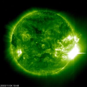
Flare of November 4, 2003 observed by the SOHO (ESA / NASA).
February 2014
The Carrington event I. - The story
Recently we were surprised by the news that the city of Boston is going to spend no less than $500,000 to buy Faraday cages, to help prevent the hypothetical effects of a high intensity magnetic storm, which is likely to occur in the near future.
Certainly, in recent years there is growing concern about this issue, due to various causes whose analysis would take us a long way (solar maximum, new means of observation such as SDO, Hollywood, ...). Now, to what extent are these fears justified? Have you ever observed something similar?
Perhaps the closest thing to this super storm is what is known as the "Carrington event", whose name encompasses the flare of September 1, 1859 and its effects on our planet.
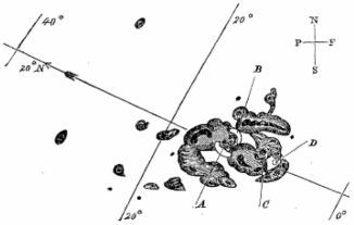
Nothing better than to let Carrington himself describe his observation:
"I had secured diagrams of all the groups and detached spots, and was engaged at the time in counting from a chronometre and recording the contacts of the spots with the cross-wires used in the observation, when within the area of the large north group (...), two patches of intensely bright and white light broke out, in the positions indicated in the appended diagram by the letters A and B, and of the forms of the spaces left white. ".
Carrington went to look for someone to confirm the observation, but on returning, the aspect had changed a lot: "The last traces were at C and D, the patches having travelled considerably from their first position, and vanishing as two rapidly fading dots of white light."
About 30 km to the north, R. Hodgson detected the same phenomenon, indicating that its brightness was similar to Vega observed with a large telescope at low magnification.
Hours later, the magnetometers in different parts of the world registered strong alterations, accompanied by auroras at low latitude, and the collapse in telegraphic communications.
Although the correlation between the solar cycle and the frequency of magnetic storms was known, Carrington was the first to identify the cause, relating his observation to the storm of the next day. Next month we will review some aspects of flare.
January 2014
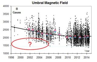
Will the spots disappear?
Perhaps one of the recent discoveries on solar activity that more rivers of ink has made run, is the "Livingston-Penn effect". These two researchers from the National Solar Observatory, have been measuring the magnetic field of the spots since the nineties, and what they observed was that the magnetic field showed a progressive decrease that did not seem linked to the activity cycle. In addition, threshold intensity measurements showed increasingly less contrasting spots, which also suggested a lower magnetic field.
If the trend continues, the magnetic field would exceed the threshold of 1500 G, and the spots would disappear in a few years, giving rise to a new minimum of Maunder.
However, the difference in behavior between the previous cycle and the current one is evident, which is showing a constant magnetic field, with no trace of decrease. Interestingly, this has delayed the expected date for the disappearance of the spots, from 2017 in the original article (2006), to 2021 in a second article (2010). Right now, the extrapolation would take us at least until 2030 at least, depending a lot on the function used ...
Recently, Nagovitsyn and Pevtsov, from the Pulkovo Observatory, have suggested a possible explanation for this effect. These researchers measure only the spot that has a greater magnetic field each day, and what they observe is a cyclic variation, synchronized with the solar cycle. In fact, this same thing appears in the Livingston and Penn graph, if we only look at the maximum values.
How to reconcile both behaviors? The existence of two populations of spots of different sizes, already detected by other researchers, could be the answer. The proportion between large and small spots varies over time, and in recent years a greater number of small spots has been observed, and fewer large spots. When averaging over all the spots, the observed net effect would be a decrease in the magnetic field.
Of course, this leaves open the question of explaining the existence of these two populations of spots, and the double dynamo effect that would originate them.
December 2013
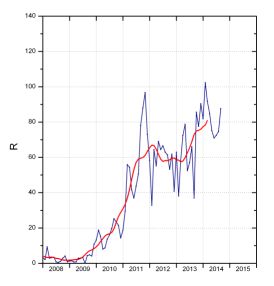
A double maximum?
When characterizing a cycle of activity, it is usual to resort to a series of parameters, such as its duration, the height of the maximum, the time of rise to the maximum, or of descent to the minimum. These parameters can convey the impression that a cycle has a smooth and uniform development, but nothing is further from reality. There are frequent ups and downs, stops or steps in the ascending or descending branch, etc ...
One feature that appears in many cycles is the presence of two maxima separated by a lower activity interval called "Gnevyshev gap". The existence of two maxima, is generally due to the north-south asymmetry. The two hemispheres of the Sun can have very different activity levels, and this asymmetry does not seem due to chance but there are indications that it responds to certain long-term patterns.
When we represent the solar cycle separating the activity by hemispheres, it can be observed that there is a lag between the two, so that one of them usually reaches the maximum before the other. It is precisely this gap that originates the two maximums, each corresponding to a different hemisphere.
According to recent studies, one hemisphere would overtake the other for 4 or 5 cycles. Then the phase shift would reverse, and the second hemisphere would reach the maximum before the next 4 or 5 cycles. Since cycle Nº 20, the northern hemisphere has advanced to the south, and this same behavior is repeating itself in the current cycle Nº 24. In future years we will have to check if the lag is reversed.
Meanwhile, the first maximum occurred in early 2012, starring the northern hemisphere. Then the activity moderated while the asymmetry was reduced. In the last months the number of Wolf seems to show a new increase, which can announce a second maximum. We'll see if this is the case, or the Sun has some surprise.
Delay in the maximums of the last solar cycles, according to hemispheres.
November 2013
Polarity reversal
Although in the Sun, the superficial magnetic fields can be distributed of very diverse forms, the polar zones are generally dominated by a unique magnetic polarity, opposite in each hemisphere, and that is inverted in the vicinity of the maximum of activity.
The inversion of polarity usually represents a milestone in the development of each cycle, although it is not something that takes place on a certain date, but rather it is a gradual process. In addition, it is usual that there is a certain lag between both hemispheres, so that they can have the same polarity for a time.
It is possible, and relatively easy with amateur media (with an H-alpha filter and a digital camera), to determine when these inversions occur, and for this the prominences can be used as markers.
One property of the prominences is that they are formed in the neutral lines that separate both polarities, so that if we have a region occupied by a polarity, the prominences will form at the edge of that area, but not inside it. This means that a measure of the latitude of the prominences can reveal the extent of that region surrounding the pole and how it decreases in size as it is replaced by the opposite polarity.
The graph shows the latitude and extent of the prominences measured in several campaigns over the last few years at the Observatory of Cantabria (the graph is similar to the Maunder diagram for spots). The red lines indicate roughly the north and south boundaries in which they appear, and in turn mark the extent of the polar magnetic regions.
The reversal occurs at the moment when the prominences reach the pole, and as we can see, that happened in mid-2012 in the north, while in the south it could be delayed until the beginning of 2014. This lag is associated with the evolution of the NS asymmetry, and the possibility that the current cycle has a maximum with double peak.
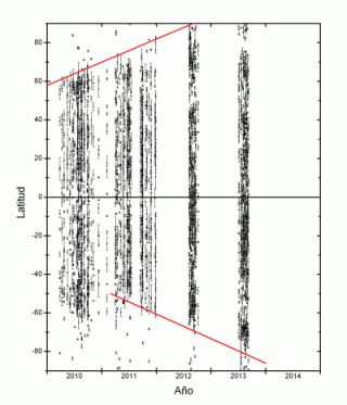
From May to October was published, divided into several parts, a summary of the article on the history of sunspots:
http://www.parhelio.com/en/articulos/artichistoria.html
April 2013
PARHELIO: A different perspective.
Of the numerous solar resources found on the internet, PARHELIO (www.parhelio.com) is a page that was born in 1999, to showcase something more specialized than what is usually done in solar observation.
Over the years, more than 60 observers have participated with their images, data, articles, etc ..., and the result of their work are, for example, the more than 52,000 Wolf numbers obtained since 1980, or the 15 years of simple observations (SV) that are collected on the page.
The development of new methods, with the use of our own software, facilitates the measurements of spots positions with errors lower than 1º; and this precision makes it possible to calculate the proper motions of the spots, their speeds and periods of rotation.
Likewise, these methods allow access, for the first time with amateur resources, to the precise measurement of the area covered by the spots, both in individual groups and in the entire disc.
The follow-up of the activity is not only done with the number of Wolf, SV, or the area. We also monitor the behavior of the asymmetry between both hemispheres, the development and evolution of activity complexes; or we create synoptic maps of the solar surface.
The activity is also recorded in daily drawings or photographs. On the page you can find images obtained during the last 20 months (about 8000), both in white light, as in calcium, or in Ha.
Other observation programs are still under development, such as the measurement of latitudes of prominences (indicative of the extension of polar magnetic fields, and the reversal of their polarity), or the detection of flares through the reception of VLF signals .
Parhelio also has a mail group (http://tech.groups.yahoo.com/group/obs_solar), active since 2002, which is made up of almost 50 members, and serves to exchange observations, news, impressions, ... . about the Sun and its activity.
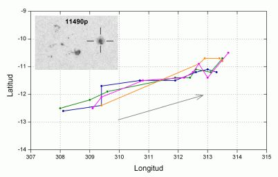
Measurements of spot NOAA11490p made by four
different observers, between May 24 and June 2, 2012.
In that interval he traveled some 70000km to more than 300km/h.
March 2013
Is this cycle so strange?
At the moment of taking the reins of this section, let us remember, briefly but meaningfully, the figure of Angel Alberto González Coroas. For years, his observations and articles showed us solar activity and its influence on Earth. His perseverance, both observational and informative, are an example for all of us.
Rivers of ink have been running for a long time about how strange the present cycle of activity is. However, in a recent article, Frédéric Clette and Laure Lefèvre, researchers at SIDC, show that with the right perspective, this is not the case.
On the one hand, what is out of the ordinary is the activity of the last cycles, much more active than the average, and it is they who are strongly conditioning our evaluation of the current cycle. Secondly, since 2000 the correlation between Wolf's number and other activity indices seems to have been broken, as if fewer spots had been counted than would be expected.
Other authors had already revealed that, comparing the last cycle (No. 23) with the previous ones, the number of groups of types C - F was similar, but there was a significant reduction in groups A and B. In light of this work, the one that is anomalous, in reality is cycle 23, and the deficit of small spots can explain its peculiar characteristics, especially in its second half.
On the other hand, during the current cycle (Nº24), the activity indexes seem to be returning to normal, and the correlation that existed between them is being recovered before the year 2000. We will have to wait for something more to see if this trend it really consolidates.