The interaction between the Sun and the Earth's atmosphere comprises many aspects. The one that interests us in the present article is to know how the solar radiation forms and models the ionosphere and the use that we can give it.

The ionosphere

The high energy radiation (mainly ultraviolet and X-rays) is responsible for ionizing the atoms of the atmosphere. However, this process does not have the same efficiency at different heights. As we go up, the radiation increases, but the number of atoms decreases. At high altitude (above 500 km), we find few atoms, so overall, the degree of ionization is small. Below about 60 km, there are so many atoms that it is easy for an ion to capture free electrons and become a neutral atom, so the ionization is not very high either.

The ionosphere extends between both heights, where ionization levels are high. As the atmosphere has a different composition depending on the height, there is no single ionization maximum, but we find several peaks depending on the abundance of different molecules. These peaks or layers are named with the letters D, E and F:

Capa F.- From 200 to 500 km. Formed by the ionization of atomic oxygen.

Layer E.- From 80 to 120 km. Formed by the ionization of molecular oxygen.

Layer D.- From 60 to 80 km. Formed by the ionization of nitric oxide and occasionally, oxygen and molecular nitrogen.

As the radiation that reaches our planet is not constant, the ionosphere is subject to seasonal, diurnal and sporadic changes. The last two are the ones that most interest us for our purpose.

The structure of the ionosphere changes with the sunrise and sunset. The D layer is only present during the day because at that height, the half-life of the ions is very small, and once the main radiation source has disappeared, they are quickly converted in neutral molecules. This process also takes place in the E layer, but more slowly, so it weakens, but normally, it does not disappear completely. Regarding the F layer, it is present at night, but by day it is usually divided into two, known as F1 and F2.

Between the sporadic phenomena, the flares suppose a sudden increase in the radiation, especially in the X-rays, which brings with it an increase in the degree of ionization, especially of the layer D. This phenomenon is known as SID (Sudden Ionospheric Disturbance)).

In addition, geomagnetic storms can also alter the properties and structure of the ionosphere, and in particular, the F layer may even disappear during these events.

Transmission of VLF signals

VLF (Very Low Frequency) signals are part of the electromagnetic spectrum and are between 3 and 30 kHz. Due to its properties, and in particular its ability to penetrate several meters of water; throughout the planet there are a series of military stations that use them to communicate with submarines, or as navigation lights.

The currents induced in the ground mean that these signals can be transmitted along the earth's surface, but this "ground wave" attenuates with a certain speed and makes it possible to detect relatively close transmitters in this way. However, it is the fact that these signals can bounce off the ionosphere which allows its transmission over long distances.

Layer D absorbs the high-frequency signals, so that they are reflected, already attenuated, in the upper layers, E and F. On the contrary, low-frequency waves can be reflected successively in layer D and on the ground, can be detected thousands of km. In this way, by day the signal is very stable. However, at night layer D disappears and the signals are reflected more efficiently in layers E and F. This means that at night, the signal usually has more intensity, although it is also more unstable. While the daytime signal is similar on different days, the nighttime signal can vary a lot. The transition between day and night is usually characterized by strong variations in the intensity of the signal.

When a SID occurs, the increase in the ionization of the D layer implies an increase in the intensity of the signal. However, the interaction with the ground wave can also cause the opposite effect.

The fact that the VLF signals modify their intensity with changes in solar radiation, is what gives us the opportunity to use them to detect flares indirectly.

In addition, there are sporadic phenomena whose cause is still unknown. As the ionosphere is very high for balloons and very low for satellites, it still has many unknowns, so it is a subject open to observation and research.

Receiving VLF signals

There are different devices that allow the reception of VLF signals. The one we describe here may not be the best, but it is certainly the simplest.

Basically, a VLF device consists of an antenna, a receiver, and a program to analyze the signal. Fortunately, the audio cards of our computers can be used as receivers, so the only hardware we need is the antenna.

The antenna.-

Numerous antenna models can be found on the internet. What we propose is a loop antenna, which can be built by winding enameled copper wire around a frame. The frame can be made with wooden slats, PVC tubes, or simply use a cardboard box.

There are three factors to consider that will influence the efficiency of the antenna: the diameter of the copper wire, the surface of the loop and the number of turns that we give to the wire.

Regarding the thread, it is not the most important factor, but it is preferable that it is thin, although in that case it will also be more fragile. It is common to use a diameter around 0.4 mm.

The shape of the loops is not important, but the surface covered by them. Keep in mind that it is about detecting wavelengths of kilometers, so the more surface better. Anyway, you can already get good results, for example, with squares of about 40 cm on each side.

As for the number of turns, we have tested antennas with about 25 laps and depending on the size and environment, they can work relatively well. However, we would recommend giving about 100 laps more or less. If the antenna is about 40-50 cm on one side, that would be between 150-200 m of copper. Although the ideal is to use a single cable, it is also possible to weld the ends of two cables to achieve a longer length.

The connection of the antenna to the computer is made through the microphone input. If we have an old microphone or headphones we can take advantage of the cable and solder one end of the copper to the input channel, and the other to ground. It is important to have a certain cable length to move the antenna away from the computer and have some freedom to locate the most suitable location.

When using the audio card as a receiver, it will be subject to interference, mainly from the power supply and other components of the computer. If the connection cable is stereo, it can be very useful to eliminate them, or at least reduce them. In this case, we will weld one end of the copper to the left channel and the other to ground, leaving the right channel free. The signal of the antenna, which includes the valid signals and some interferences, plus those interferences created directly on the cable and the card, will enter through the left channel. The right channel, which we have left free, will receive only the latter. With the program that we use, we can subtract both channels and leave the signal much cleaner.

The location and orientation of the antenna are crucial factors. Sometimes, a few meters are the difference between a good and a bad reception. Obviously, the center of a city is not the most ideal place to install our station, but even so, in those conditions it is possible to register and measure the most powerful stations.

Our antenna is directional, detecting more effectively the signals that arrive perpendicular to the plane of the turns. However, the proximity of metal masses or the orography itself can cause signals to arrive from unexpected directions. As an example, in some places we have only been able to detect British stations with the antenna oriented in the E-W direction (!).

Software .-

Once our antenna is built and connected to the computer, we will need a program to help us visualize and measure the signals. As with the antenna, on-line you can find various programs that carry out this work. For being free, in what follows we will refer to Spectrum Lab, although any other would be useful, as long as it allows to measure the intensity of a signal over time. The program can be found at the following address: http://www.qsl.net/dl4yhf/spectra1.html

The program has many options and possibilities to work with signals, and it would be very long to describe all the tests we have done until we find the configuration that best seems to work. Also, unfortunately, the tutorial seems written for people with previous knowledge of electronics, radio, and signal processing. Therefore, we will simply list those options that give us the best results, although of course, it is possible that with different computers, antennas, locations, etc ... other optimal configurations could be found.

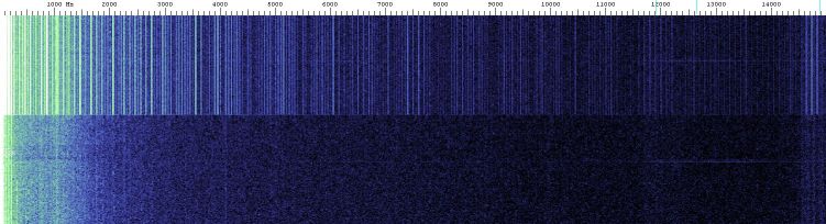
The main window of the program has a superior graph where the spectrum of the signal received by the audio card appears (X = frequencies, Y = intensity). The peaks may be emitters, interferences or background noise. The interferences appear as narrow and very defined peaks, which are usually repeated at regular intervals, mainly 50 or 60 hz (frequency of alternating current in Europe and America respectively). The stations usually appear as bands that can be more than 100 or 200 hours wide.

Below is another graph that shows the evolution of the spectrum over time as a waterfall (X = frequency, Y = time).

On the left we see some options. For the moment, clicking on the color palette will choose the one that seems most appropriate. This has some importance because it can facilitate the visibility of weak stations.

Next we will describe how to configure the program in two different ways: with a filter, or in stereo mode. The objective that we pursue with the following options is to achieve a spectrum as free as possible of interference, where the signals have a smooth Gaussian profile. The intensity measurements should show little dispersion, except logically, due to natural causes.

The fluctuations of the signal that we are interested in eliminating may be due to interferences or to variations in the background level (in the last instance, also due to interference). The filter works very well on the interference peaks, but it barely acts on the background, so it is the best method if we want to measure the most powerful stations, discarding the weak ones, which will be very affected by the background. The stereo mode corrects relatively well the variations of the background, and only partially the peaks of interference. It allows using weaker signals, but the dispersion of the data is greater than with the filter. All this is valid if we are in "urban" conditions. In a place away from sources of interference, surely we do not need any of the two methods to get a clean spectrum.

It is important to have a good spectrum before starting to measure. Therefore, for now we will not look at the intensity graphs; we will only pay attention to the spectrum or the waterfall. Only when we have a spectrum as free of interference as possible, will it be time to start getting measurements and check the dispersion of the data.

- Configuration with filter.-

This configuration can be used with a mono or stereo cable, interchangeably.

- Quick Settings menu, Load & Create user-def'd entries.- We chose the VLF_Stations.usr file as a starting point. Later, when we finish configuring the program we can save this configuration with another name, in the File menu, Save Settings as. The file that we have opened extends the spectrum to 22000 Hz and marks the frequencies of different stations on the upper graph.

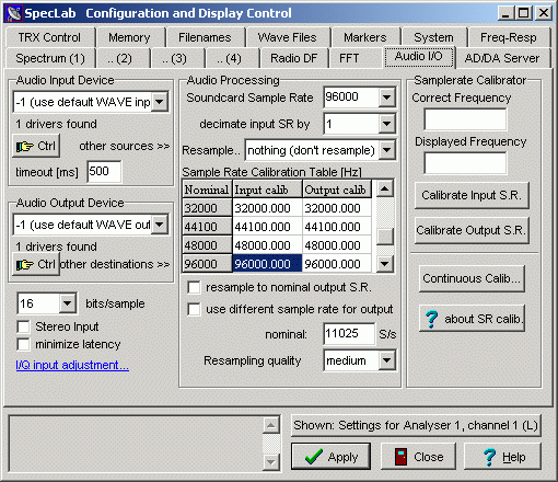
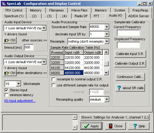
- Options Menu, Audio Settings.- On the Audio I / O tab, the most important parameter is the Soundcard Sample Rate. The maximum frequency we can observe is half this value (Nyquist frequency). We must also bear in mind that, depending on the model, the audio card only samples up to a certain frequency. A suitable value can be 48000. To observe a station that emits in 46000 hz, for example, it would have to raise it to 96000 or 192000, if the card allows it (see note at the end).

On the left we can leave the Audio Input and Audio Outpout in their default values, and below, let's make sure we're using at least 16 bits / sample, and that the Stereo input box is unchecked:

- Spectrum (1) Tab.- In Waterfall Scroll Interval, we will uncheck Automatic, and in the box we will say 1 sec. If above, the option Optimal waterfall average is checked, each line of the waterfall will be the result of adding all the possible spectra obtained in an interval of 1 sec. Of course, we can increase or decrease its value and with that, we will modify the cascade speed. A very small value is not recommended so as not to overload the CPU, especially if we use a high resolution.

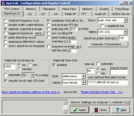
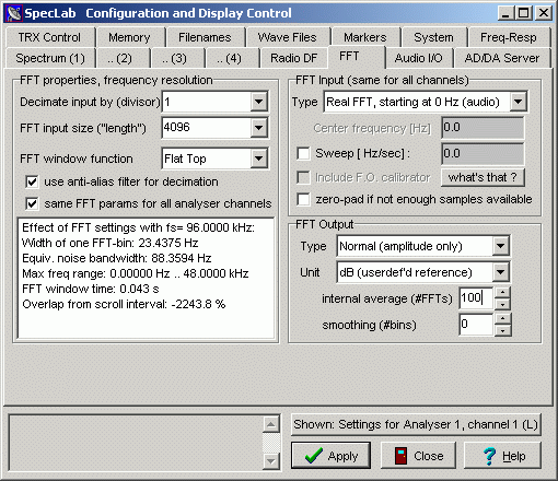
- FFT Tab.- FFT Input Size determines the resolution of the spectrum. At the beginning we will set a high resolution (32768, for example), to see the interference peaks and adjust the filter parameters. Then we will download it to make the measurements.

The value in the "Internal average" and "Smoothing" boxes must be zero for the moment.

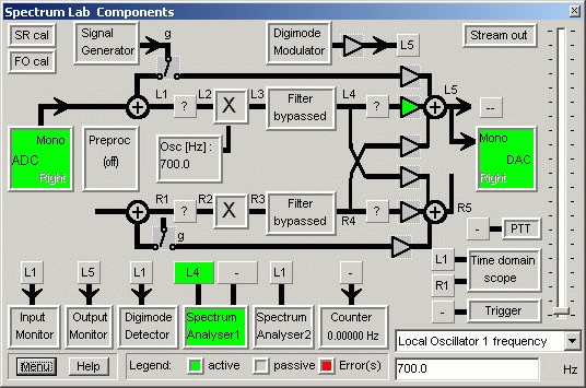
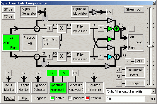
- Components Menu, Show components.- The window that appears shows a circuit diagram, where you can configure the different treatments that you want to apply to the signal. If we use a stereo cable, the upper half corresponds to the left channel (L1 ....... L5), and the lower one to the right (R1 ....... R5). If we click on the different boxes, a series of windows and menus with numerous options appear. At the beginning, it is preferable that we deactivate all treatments.

On the left, the ADC box must have only the left channel activated. Below we will see the "Spectrum Analyzer1" box connected to two others. On the left you have to put L4 and the right to leave it empty. The window has to look like this:

Now we click on the "Filter bypassed" box between L3 and L4, and the filter configuration window opens:

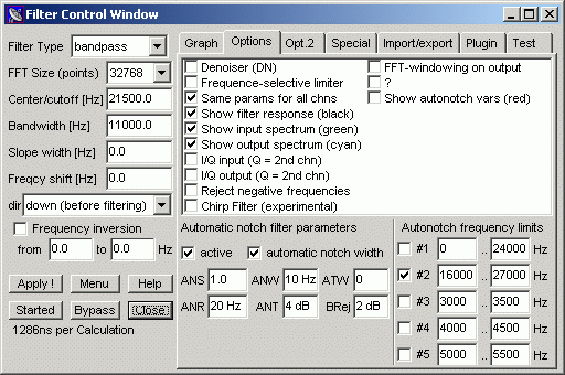
Actually we are going to use two filters; one general, to select the area of ​​the spectrum that interests us, and another called "autonotch" or "automatic notch", which will act on the interference. As the peaks we want to eliminate have a bandwidth of a few Hz, it is convenient to use a high resolution in FFT Size. Otherwise, the filter will hardly notice variation between a "pixel" and the adjacent ones, and when it does (precisely in the stations), it will also act on the signal.

The parameters "Filter type", "Center / cutoff", and "Bandwidth", are what determine the area of ​​the spectrum that we are going to see. With the values ​​of the image, the filter blocks the entire spectrum except for a band between 16000 and 27000 Hz, which is where the main stations are located.

The autonotch filter basically compares the intensity of each "pixel" of the spectrum with the adjacent ones, and if the intensity exceeds the average, cancels those frequencies. The most important parameters are ANS, which determines the intensity of the filter; ANR, which defines the width of the region that will be used to compare; and ANT, which is a threshold intensity, so that only the peaks exceeding this intensity are eliminated.

The values ​​of the image have given us good results, but each one must try to obtain the best results with its spectrum. Once we have found the right values. click on the Menu button, Filter running; then on the buttons Stopped (will change to Started), Bypassed, and Close. We'll see that the Filter box turns green, and we'll check the effect of the filter on the waterfall.

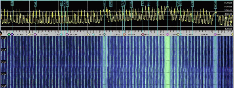
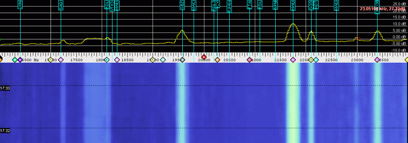
In the following image you can see an area of ​​the spectrum without the filter (above) and with the filter (below).

Once the spectrum is clean, it is better to change some options to perform the measurements. Again, we go to the Options Menu, Audio Settings, FFT Tab. We lower the resolution to 4096 (if the sampling rate is 96000), or 2048 (if the sample rate is 48000), and we choose "Flat top" as FFT window. The Smoothing option performs a kind of moving average on the frequency axis, smoothing the spectrum, but at the expense of introducing an adjacent signal to the one that interests us, so it must always remain at 0.

Internal Average averages as many spectra as we indicate in the box, so that it smooths the variations in the time axis. This option is equivalent to smoothing the graphs later and you have to play with different values ​​to decrease the dispersion of the data, but without exceeding it, so as not to eliminate real variations.

In the window appears a series of information, in particular the "FFT window time", which is the time it takes to calculate a single spectrum. The Internal average will depend on that time and the temporary resolution that we are using. For example, suppose that in the graph we represent a data per minute, and we want to average all the spectra obtained in that minute. If a spectrum is obtained every 0.043 sec, the Internal average will be about 1400. There is no problem in using such a high value, since the SIDs usually last much longer.

Perhaps due to an error in the program, the maximum value that appears in the box is 100, although it accepts higher values. If we enter the value 500, when clicking on Apply, the value will change to 100, but the program will use 500. If we want to use a value >100, we must always enter it before clicking Apply, even if we are doing tests with other parameters.

Once these parameters are entered, we are ready to take measurements (see below).





- Stereo configuration.-

This configuration can only be used with a stereo cable.

- Quick Settings menu, Load & Create user-def'd entries.- Same as the configuration with filter.

- Options Menu, Audio Settings.- Same as the filter configuration, but checking the Stereo Input box.

- Spectrum(1) tab.- Same as the filter configuration. On the right, in Maths we choose CH1 - CH2.

- FFT Tab.- FFT Input Size determines the resolution of the spectrum. You have to look for the best value; in our case: 2048, if we are sampling at 48000. If we put the sample at 96000, then we will have to go up to 4096, to maintain the same resolution. In FFT window function we choose Flat Top.

Regarding the Internal average and the Smoothing, the same recommendations that we saw above are valid, that is, Smoothing = 0, and Internal average obtained by experimentation.

- Components Menu, Show components.- The window that appears shows a circuit diagram, where you can configure the different treatments that you want to apply to the signal. The upper half corresponds to the left channel (L1 ....... L5), and the lower half to the right (R1 ....... R5). If we click on the different boxes, a series of windows and menus with numerous options appear. At the beginning, it is preferable that we deactivate all treatments.

On the left, the ADC box must have both channels activated, checking the Stereo mode option. Below we will see the "Spectrum Analyzer1" box connected to two others. On the left we can put L1 and on the right R1. If we have deactivated all possible treatments, we can also put L4-R4, or the intermediate steps. The window has to look like this:

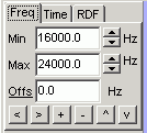
- In the main window of the program, in the Freq tab there are several buttons that allow you to zoom or move through the spectrum. We can also set a frequency range by filling in the Min and Max boxes.

When subtracting the channels, the intensity is going to go almost to 0 db, so we will have to move so that this value appears in the upper graph, to the right.

On the other hand, if we have a cathode ray tube monitor nearby, we will see a very pronounced peak at 15600 Hz and another at 31200 Hz, which will contaminate a large part of the spectrum. Fortunately, between both there is an area where some interesting stations can be received to follow up. Therefore, it is good to establish the frequency range between 16000 and 24000 or 25000 hz.



The following image is an example of a spectrum with a serious problem of interference, obtained only with the left channel and without any treatment. In this case, we have used a high resolution to appreciate the interferences well. However, even in such unfavorable conditions we have been able to detect fugurations:

This other image shows the effect of the configuration that we have described previously, with the same equipment and in the same location:

Measurement of intensity

Once you have achieved a good visualization of the signals, you have to measure their intensity and see how it varies with time. To do this, go to the View / Windows menu and mark Watch List & Plot Window. In the window that opens, Watch List tab, we can see a list of the channels that will be represented in the graph. You can modify the contents of the boxes simply by clicking on them.

- Nr.- Is the number of each channel and the color assigned in the graph. To modify the order, we can click on a channel and drag it up or down.

- Title.- An arbitrary name that we will assign to each channel to identify it.

- Expression.- It is the most important because it tells the program what it has to represent. We will use 2 functions: noise_n, and avrg_n; the first calculates the noise and the second the average, all in the specified frequency range. In both cases, normalizes the result to a bandwidth of 1 hz.

The function that comes by default for the signals is peak_a, which calculates the maximum intensity in the intervals of frequencies and time considered, but it does not work because it is very sensitive to noise and variations in the background. With the signals we will use avrg_n, and with the noise, noise_n.

The two figures in parentheses indicate the frequency range where the calculation will be performed. In the case of noise, this interval must be at least 5 times greater than that of the corresponding signal. For example, if we are measuring a signal in the interval (19550,19650), the interval for noise must be at least (19350, 19850). The noise measurement is not mandatory, but it can serve as a reference to know if the variation of a signal is real, or is due to a change in the background intensity.

- Result.- It is the value of the function calculated at that moment.

- Format.- The format with which the results will be written.

- Scale Min, Scale Max.- These are the minimum and maximum values ​​that will appear in the graph. As due to the treatment of the signal, we have the background intensity close to zero, we can put a minimum of -5 or -10. The maximum will depend on the intensity of the signals. A change in these two columns will only take effect after closing and opening the window again.

If we are measuring several channels, all of them will appear almost superimposed on the graph, making visualization difficult. To see them separated, we can add or subtract a constant to the function, in the Expression column.

The Layout tab is used to configure some aspects of the graph.

In the Horizontal tab, the Scroll Rate box allows us to control the speed at which the data appears in the graph, while defining the time interval in which the functions represented in it are applied.

The Channels & Colors tab allows you to configure the curves associated with each channel, assigning them a color and a line type. In the lower part, we can choose to represent the minimum, maximum or average value within the previously selected time interval. There should not be much difference, so the average can be fine.

In the Memory tab, Misc., We indicate the number of channels that we are going to measure. The data is stored in the memory of the program and is preserved even if we close it. The Samples box allows you to indicate the extension of the memory. For example, if you represent 1 data every minute, a value of 5000 in the box indicates that you will store 5000 minutes per channel, that is, about 3.5 days.

Finally, the Export tab is used to tell the program how to export the data to a text file. It may be important to check the "Periodically export ....." box so that you can write the data in real time. In that way, we avoid losing them in the event of a program failure.

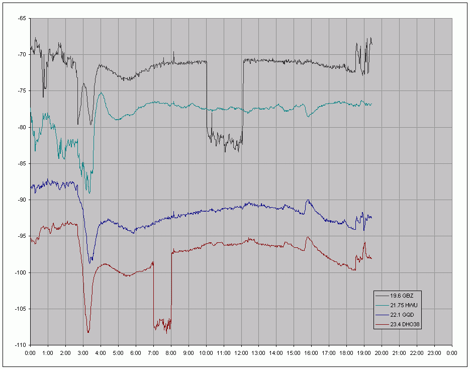
The following chart is an example of what can be recorded. It includes the signals of 4 stations and the effect of two flares registered at 1430 and 1545 can be seen. Another weaker one is also predicted at 1215. The fades of the signal in GBZ and DHO38 are disconnections that occur occasionally for maintenance reasons.

Station list

In the following links there are listings of the stations that can be found in these frequencies:

http://sidstation.loudet.org/stations-list-en.xhtml

http://www.vlf.it/trond2/list.html

http://df3lp.de/misc/freq-list.html

http://www.smeter.net/stations/stations.php

http://www.mwlist.org/vlf.php

You have to be proving when it comes to identifying stations, because everything that glitters is not gold. Sometimes there may be an interference in the frequency corresponding to a station, so always check that the signal has the expected variation.

Javier Ruiz

Note for Windows 7 users

Windows 7 has a mechanism for sharing recording devices in different programs. This mechanism 'tricks' the programs, making them believe that they have reserved the audio adapter for their use. Thus, when a program wants to capture audio, you must always specify the capture format - for example, the sampling rate. Windows 7 lies making the program believe that it has been able to configure the speed, but in fact Windows has already opened and decided on the sampling format, and is dedicated to revamping the data it sends to each application allegedly in the format they requested.

This has the advantage that you can have several programs capturing sound from the same source at the same time. The downside is that if, for example, we set the sampling rate to 48000, Windows 7 will not say no if, for example, Win has the device open to 44100. How does it work? Duplicating samples up to 48000. This makes the application believe that everything is on wheels, but if we make a spectrum, the collateral effect is that, from the Nyquist frequency corresponding to the actual capture frequency, it will be reflected a mirror of the existing signal, up to the new fictitious cutoff frequency.

In summary, in Windows 7, if we set the sampling to 48000 or higher, we must determine if from the frequency 22050 of the spectrum a mirror split of the signal immediately below is observed. If so, it is that Windows 7 is sampling at 44100 and filling holes on its own. The solution is to go to the control panel, in the window finder write 'audio properties', and in the recording properties tab specify the exact recording format that we are going to use in our program. So Windows will not have to invent anything and everything will go smoothly.

Daniel Gracia