The Sun has polar caps, but logically they are not occupied by ice but by magnetic polarity. Each of them contains a unique polarity and most of the time, the polarity in the north is opposite to that of the south. Only during the maximum of the cycle it can happen that both have the same polarity, depending on the lag in the activity of the two hemispheres.

During the minimum of the cycle, coronal holes can be observed on both caps. In figure 1, on the left, we have the situation during the minimum, with two wide holes well defined.

Figure 1

The magnetic fields in these zones are controlled by the emersion of active regions near the equator. The magnetic field originating in the spots f travels toward the pole more efficiently than the p, and being of opposite polarity subtracts the one that occupies the polar regions by decreasing its intensity. The temporal evolution of the polar regions depends on this mechanism. During the minimum cycle the caps reach their maximum extension. When the new cycle begins and the number of groups increases, the polar magnetic fields are diminished, and the caps gradually reduce their size. At maximum activity, the magnetic fields cancel out and the caps disappear. This situation can be seen in Figure 1, in the image on the right, obtained four years before the previous one, during the maximum. From that moment, the polarities are inverted and the caps reappear.

With the means at our disposal we can observe two phenomena associated with this process, which inform us about the extension of the caps and the intensity of their magnetic fields, allowing us therefore to follow their evolution. It is the prominences and the polar faculae.

PROMINENCES

The main characteristic of the prominences is that they are formed in the neutral line that separates both polarities. If we have a large region occupied by a single polarity, as in the case of a polar cap, the prominences will form in its periphery, but not in its interior. This means that in a minimum of activity we will not observe prominences at the poles; the maximum latitude at which they form will coincide with the one with the cap limit. In fact, in this phase of the cycle, a crown of prominences can sometimes be observed surrounding the polar regions (Figure 2).

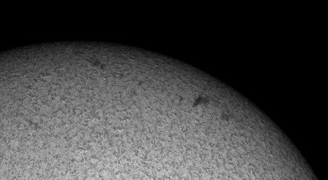
Figure 2

When the cycle begins and activity increases, the prominences follow the reduction in the size of the cap and appear more and more latitude. At the maximum, the prominences reach the pole and it is when the polarity reversal occurs. Due to the lag in the development of the activity of both hemispheres, the prominences in the north and the south are generally not synchronized, that is, they do not have the same maximum latitude nor reach the pole at the same time

From all the above it follows that simply by measuring the latitudes of the prominences we can know the extent of the polar caps, follow their evolution and even know when the inversion of the global magnetic field occurs.

As usual, we do the measurements through the SOL and Iris programs. The treatment of the images is similar to the one we use to measure stain positions, although it presents two evident differences. The first is that the images must be obtained with an H-alpha filter, and the second is that now a treatment is done for the interior of the disc and another for the outside, because it is in the limbo where we are going to make the measurements. Once the limb image is obtained, we mark with the cursor the north and south ends of each prominence and in the Iris Output window, the coordinates (x, y) of each point appear in the image. When finished, SOL accesses these data and calculates the average latitude and dimensions of each prominence. Details can be found in the SOL program instructions: http://www.parhelio.com/en/docsoftware.html

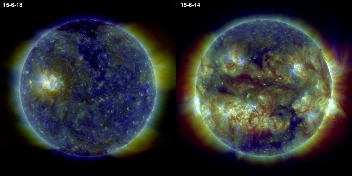
As an example, in Figure 3 you can see two images obtained during the process and representative of two moments of the cycle, one corresponding to the minimum (2018) and another to the maximum (2014). While in the first, the maximum latitude reached by the prominences is around 50º-55º, in the second it can be seen that they reach the polar regions.

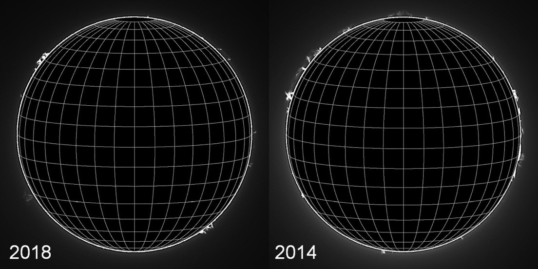
Figure 3

POLAR FACULAE

Already in the nineteenth century, several observers noticed the existence of two types of faculae. The most apparent are formed in middle and low latitudes and are associated with active regions. However, others appear in the polar regions, and they are small and short-lived. In general, the telescope appears as bright spots and generally with a fairly low contrast, although exceptions can always be found. Given its characteristics, good image quality is needed to observe them properly. In addition, its visibility depends on the inclination of the solar rotation axis. In September faculaes will be better seen in the north, because that pole tilts towards the Earth, while six months later the situation will be the reverse and the southern faculae will be better detected (see http://www.parhelio.com/en/doccoord.html).

Since the faculae appear in those areas where there is a greater magnetic field, their number gives us information about the intensity of the polar magnetic fields, and their evolution goes in parallel with the solar caps. They are more numerous in the minimum activity, when the caps are more extensive, and practically disappear at the maximum of the cycle. Of course, there will also be an annual variation that, as we have seen, depends on the orientation of the axis of rotation.

To track the polar faculae, we use the same images as to measure the positions of spots or the total area, that is, images of the entire disk properly oriented, with the solar north above. However, although these images can be used without any additional treatment, the faculae appear with an aspect similar to that which they visually have through the telescope, and therefore, with a rather low contrast. Therefore, it is important to make certain modifications that facilitate its detection and measurement. The following procedure is carried out almost automatically using the software Iris and SOL.

The first step is to eliminate the limb darkening. This will allow to increase the contrast without the variations of intensity of the background supposing a limitation. In figure 4, on the left we have an original image, and on the right, without the limb darkening. In figure 5 we can see the north polar cap of both images, where it can be seen how the faculae, barely visible in the first, can be seen more clearly in the second.

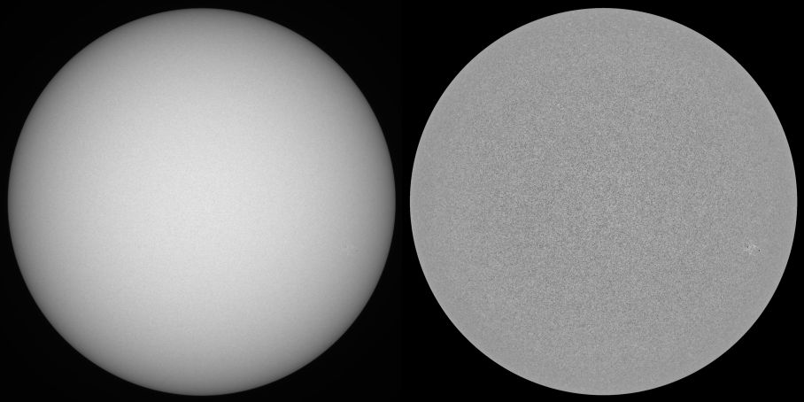
Figure 4

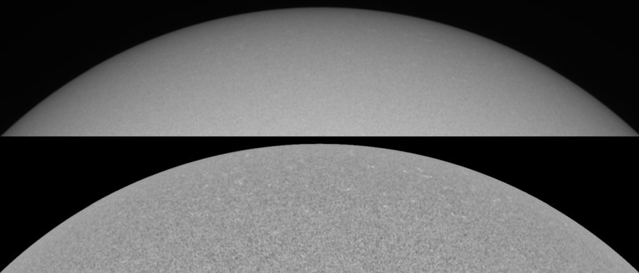
Figure 5

Iris allows to make a series of changes of coordinates to show an image of the whole disk in different cartographic projections. One of them is the polar stereographic projection, which will be especially useful. In it, the points of a sphere are projected on a plane tangent to one of the poles, using as vertex the opposite pole. Its main property is that it preserves the angles and shapes, so that the distortion it introduces is small, at least up to mid-latitudes. The resulting image shows a cap as if we were located on the pole, and the semicircle shape corresponds to the hemisphere visible from Earth (the hidden hemisphere would be at the top). The images we use have a latitude range between 50º and 90º, and over them we superimpose the central meridian and the parallels in 10º intervals. Figure 6 shows the polar projection of the north cap corresponding to the example image we are using. The visibility of the faculae is much higher, and by eliminating the effect of the perspective near the limb, its measurement and monitoring is greatly facilitated.

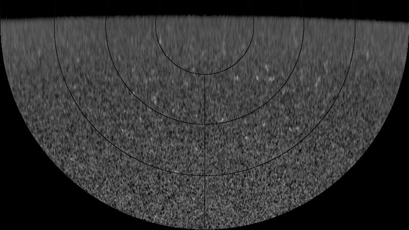
Figure 6

The observation of the facula will depend on two factors: the quality of the images and the criterion of the observer. In good images the faculae are almost punctual and more extensive details seem formed by association of several faculae. In medium quality images we will lose the faculae weaker and the rest, appears larger and with a blurred appearance due to seeing. The images of worse quality are better to discard them.

The criterion of the observer influences when determining what is or is not a facula. With the smallest or weakest details there will always be doubt about whether they are really faculae or it is simply noise or a granulation effect (granules or association of granules slightly brighter than the environment). This factor will appear as a kind of "bias" so that one observer will systematically register more or less facula than another.

However, both factors will have a relative importance because if we do counts, we are not interested in absolute values ​​but in their temporal variation, and in addition, we will work at least with monthly averages. On the other hand, if we measure positions, what will be relevant are the regions with the highest density of faculae and how they evolve over months or years, and not the background activity, which is much more dispersed.

In Parhelio we obtain two types of data: positions and number of faculae. With the software usual, SOL and Iris, the positions of the faculae can be obtained quickly and easily. During the treatment of the images of the whole disk, both programs can automatically obtain the polar images. Once opened in Iris, the contents of the Output window are erased and all the faculae are marked with the cursor. In the Output window, the coordinates (x, y) of each facula appear. Once we finish, SOL will read the contents of the window and with that data, get a list with the heliographic coordinates. This method is not as precise as the one we use with the spots, but we must not forget that we are close to the limb and using the minimum or maximum photometric does not guarantee that we will obtain great precision.

Regarding the counts of the number of faculae, it can be done in two ways: directly on the images or using the position measurements. We have verified that with the measures of position some higher values ​​are obtained, perhaps because it tends to be more meticulous and pay more attention to the small facula. The insertion in the images of parallels every 10º, also allows to realize counts by intervals of latitude.