SOFTWARE |
SOL
Installation.-
You have to download the sol.rar file and unzip it into a folder. The program does not install any additional files or modify the registry.
The compressed file includes the executable, a library for algebraic calculations (algibnet2.dll), a library for the calculation of ephemeris (vsop.dll) and the documentation of the program.
To uninstall, simply delete the folder where the executable is located.
System Requirements.-
- Microsoft .NET Framework 3.5 SP1
If it is not installed, it can be done from: https://www.microsoft.com/es-es/download/details.aspx?id=30653
License.-
This program is distributed without a license or guarantee of any kind. Its use is made under the sole responsibility of the user.
To report any error of the program you can write to the address parhelio@astrocantabria.org indicating in the most accurate way possible what type of error it is, at what exact moment it occurs, and sending the check.txt file that will be found in the working folder. Eventually, additional files may be requested to try to identify the cause of the error and its possible solution.
Introduction.-
The measurement of positions from photographs is done with the Iris program, according to the method described in the following web page:
http://www.parhelio.com/en/docposicfotos.html
Iris can be downloaded at the following links, in its French and English versions:
http://www.astrosurf.com/buil/us/iris/iris.htm
http://www.astrosurf.com/buil/iris/iris.htm
The procedure is long and for this reason, SOL was initially designed to automate certain tasks (especially the orientation of the image).
Subsequently, the program was extended to allow the measurement of positions with a reticle, areas, different geometrical parameters of the prominences, as well as the calculation of ephemerides and proper motions of spots.
In its current state, SOL works as a virtual user of Iris, making the process of measuring positions almost totally automatic.
The advantages are obvious. In the first place, it is hardly necessary to know how Iris works. However, since in most of its functions, the program was thought to work in conjunction with Iris, it may be convenient to have a certain familiarity with the working methods of this program.
On the other hand, the method is included in the code. This ensures that all observers use the same method, and that the influence of the observer on the result is minimal.
Also, the process is very fast. In a few minutes you can get a whole set of measurements from a sequence of several dozens of images.
In Parhelio you can find more detailed information about the processes carried out with Iris.
Configuration.-
First of all it is necessary to configure some parameters, depending on the part of the program that we are going to use. If we are only going to use the program to generate ephemeris or proper motions, it is not necessary to configure anything.
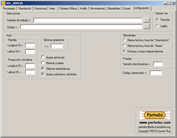
The first time we open it, the program will create the file "sol.ini" with some default values. To modify them we go to the "Settings" tab and there we enter the following data:
Addresses:
- Work folder.- Here we must put the address of the work folder of Iris. Given the interaction between Sol and Iris, it is convenient that both share the same folder.
- Scripts.- To perform some functions, SOL uses the ability of Iris to work with scripts. Here you should see the same address that Iris uses to store the scripts.
Template:
- Size of the image (pixels) .- We must enter the horizontal and vertical dimensions of the image, in pixels. These dimensions are constant for each camera model. If we load an image in Iris, the command >info, will provide us with these dimensions. You have to use the values of Iris, not those that come in the specifications of the camera, since sometimes they do not match.
- Intervals of longitude and latitude (º) .- When Iris draws a template on the disk of the Sun, these values provide the space in degrees, between meridians and adjacent parallels. An adequate value in most cases is 10º.
Code:
- Observer code.- The 3-letter code assigned in Parhelio to each observer.
Areas:
- Pixel size (micrometers) .- The size of the camera pixels in micrometers. This information is usually found in the camera's documentation. The data is also used in calculations on prominences.
It is necessary if we are going to measure areas of individual groups, but if we only want to obtain the total area measured on an image of the whole disk, we can do without it. The data is also used in calculations on prominences and the Wilson effect.
Ephemeris:
The date and time can be entered in the Processed, Area, and Ephemeris tabs. Since the ephemeris module can be used in combination with the other two, we can choose if we want the data entered in Processing or Area to appear automatically in Ephemerides, or if we want the tabs to remain independent of each other.
The option that we mark will only be effective after restarting the program.
Auto:
- Iris version.- Indicate if we are using the French or English version.
- Background adjustment.- (Only for users of Canon digital cameras). With the treatment carried out by the program, the images obtained by Canon cameras are little contrasted and the background very bright. Checking this box makes an automatic level adjustment that darkens the background and increases the contrast. The setting applies only to the resulting bmp images.
- Eliminate gradient.- The limb darkening depends on the wavelength, and we need to know it in order for the elimination to be effective. In a digital camera a suitable value can be 550 nm.
- Cylindrical projection.- During the process to eliminate the limb darkening, the program has the option of passing the image to cylindrical projection. The values entered here are used to trim the resulting image. With Length = 180 and Latitude = 90 (maximum values), Iris shows the entire solar surface, so half will appear black. With values Length = 70 and Latitude = 60, the program shows the surface at +/- 70º of the central meridian and at +/- 60º of latitude.
- Obtain statistics of the sequence.- Before aligning and adding the sequence of images, there is the possibility of obtaining a statistics of the same. This can be used to know the goodness of the sequence. If the box is checked, the values of the mean and median are displayed later on the Orientation tab.
- Polynomial fit of limb.- This option is always checked by default. To determine the intensity of the limb, SOL uses a polynomial fit. If when using the "Align (2)" button the program encounters problems when obtaining the intensity of the limb, this box can be unchecked and the process repeated. In that way, a different method that could solve that difficulty will be used. This option has effect only with the "Align (2)" button.
Important:
- The hours are entered in "hhmm" format. For example, 13h 56m should be written as 1356.
- While Iris performs some process such as aligning, orienting, or eliminating the limb darkening, SOL is minimized to the task bar, reappearing once the treatment is finished.
- When Iris executes any of the scripts, sometimes the message "Does not answer" appears in any of its windows. It is enough to wait until the process finishes and the SOL window reappears in the foreground.
- By eliminating the limb darkening, at the moment of synthesizing the background, Iris can emit a sound, as if an error had occurred. It is also normal and the treatment will continue without problem.
- The calculation of the statistics lasts a few seconds during which it seems that the program does not do anything, but that does not mean that it has been blocked.
- During the processing of the images, SOL creates the check.txt file. In case of any error, the data it contains may be useful to identify the cause of the error.
Treatment of images
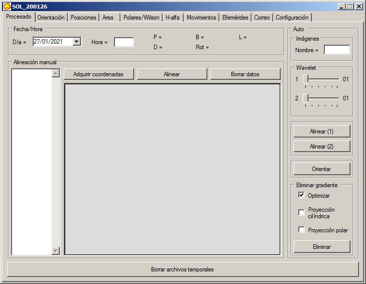
The window is divided into two main parts: Manual alignment and Auto. The latter is the section that we will use under normal conditions.
The starting material is a sequence of images of the entire disc, obtained without tracking. Previously, with Iris, we will have passed the raw format of the camera to fit format.
First of all, it is necessary to enter the date and time of the observation (those corresponding to the central image of the sequence). The program will calculate the ephemeris for that moment:
P.- Inclination of the axis of solar rotation, with respect to the N-S direction.
B.- Heliographic latitude of the center of the solar disk.
L.- Heliographic length of the central meridian.
D.- Solar diameter in seconds of arc.
Rot.- The number of solar rotation. The decimals indicate the fraction of the rotation in which we are.
SOL can use three alignment methods. Choosing one or the other will depend on the characteristics of the sequence.
 |
 |
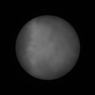 |
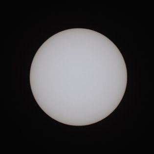
1.- The first image corresponds to a sequence carried out under optimal conditions (clear sky and stable transparency during the duration of the sequence). The disc is well contrasted and the pixels corresponding to the limb have a similar intensity, both in each individual image and throughout the entire sequence. You can adjust a circle to the limb of an image and use that same intensity to make the adjustment in all the images.
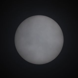
2.- The second image belongs to a sequence obtained through high clouds. The intensity of the pixels corresponding to the limb in each image separately, is approximately equal, but can vary quite a lot along the sequence. You can adjust a circle to the limb of each image, but you can not use that intensity to make the adjustment in the rest.
3.- The third sequence is affected by dense clouds. The pixels corresponding to the limb have very different intensities, both in each image and in the whole sequence. You can not fit a circle to the limb.
Let's see how to act in each case.
Auto.-
This module allows to almost completely automate the work with Iris from a few starting parameters. However, it also needs very precise conditions, which if not met can cause errors or interrupt the process:
1.- Iris does not have to be minimized in the taskbar, although it is not necessary to be in the foreground.
2.- In Iris, the command window and the output window should be open
3.- In the command window, the last line must have only a ">" sign.
4.- Before starting the processing, both in white light and H-alpha, it is convenient that in the work folder there are no images created in previous treatments. You can use the "Delete temporary files" button to delete them.
In "Auto", we put the generic name of the images and we can indicate if we want to apply wavelets. Cursor 1 will highlight the layer with the finest details, and 2, the next. If we leave them to the minimum, the program will skip that step.
Although usually do not modify the photometric center, it is advisable not to use wavelets unless it is necessary, in case there are very faint spots, for example. It is always possible to apply wavelet later with Iris, from the image "k.fit" that will be created in the work folder.
In case of using them, it is necessary to do it with prudence and not to introduce very high values, because it is easy to introduce artifacts that later affect the elimination of the limb darkening or the calculation of the area.
++++++++++++++++++++++++++++++++++++++++++++++++++++++++++++++
Suppose we have a sequence performed in good conditions, like the one in the first image.
Once verified that all the above conditions are met, click on the "Align (1)" button. The operations performed by this button are the following:
- Obtain the statistics of the sequence, if we have indicated it in the Program Configuration. This step may take several seconds.
- Calculate the intensity of the limb in the central image of the sequence.
- Use that intensity to adjust a circle to the Sun's disk in all images, and align from its centers.
- Add and obtain the center and radius of the disk of the resulting image.
When finished, the program window reappears with the Orientation tab selected. If we see that everything is correct (see below), we return to the "Treatment" tab, and click on the Orient button. The operations performed by this button are the following:
- Rotate the image and if necessary, invert it to place the solar north above.
- Adjusts the histogram.
- Calculate the center and radius of the disk of this new image.
- Repeat the calculation of the center and radius correcting the influence of very dark spots.
- Create a text file with the parameters that define the coordinate network. The file is called sol.lst and it is saved in the working folder.
- Apply wavelet if we have indicated it.
- Fix the background if we have indicated it in the configuration.
- Crop and save in bmp format, two images of the oriented disk, one with the superimposed template and one without it.
It is convenient to examine the image of the template to verify that it effectively fits the limbus well. Then, we can go to the "Positions" tab to make the measurements.
In white light, once the positions are measured, we can eliminate the limb darkening by following the steps described in: http://www.parhelio.com/en/doctecnicas.html
The process consists of two phases. In the first, a disk with the gradient corresponding to the wavelength used is created, and subtracted from the image. The second phase optimizes the result by adjusting residual gradients and correcting them.
The "Optimize" box is always checked by default, and it is important to leave it that way because almost always, optimization produces a better result. However, exceptionally, it can generate additional gradients. If that happens, we uncheck the box and click again on Delete.
If the box "Cylindrical Projection" is checked, at the end the program will also pass the image to cylindrical coordinates and save it in bmp format. The image will have a scale of 0.1º / px and can be used to make planispheres. The Longitude and Latitude boxes on the Configuration tab set the limits of this image.
On the other hand, checking "Polar projection", we obtain two images of the poles of the Sun, the north on the left and the south on the right. Both cover the zone between 50º and 90º of latitude and the central meridian and the parallels to 60º, 70º and 80º are superimposed on them.
This type of images are used to register polar faculae. However, because they are small features and low contrast, to appreciate them it is necessary that the original images have been obtained in good condition and with sufficient resolution.
++++++++++++++++++++++++++++++++++++++++++++++++++++++++++++++
Now suppose we have a sequence like the one in the second image, where you can not use the intensity of an image to align the rest.
Here we will use the "Align (2)" button, which performs the following operations:
- Obtain the statistics of the sequence, if we have indicated it in Configuration. This step may take several seconds.
- For all the images in the sequence, calculate the intensity of the limb, adjust a circle and obtain the coordinates of the center of the disk.
- With the centers, the file Shift.lst is created, which is used to align the sequence.
- Add and obtain the center and radius of the disk of the resulting image.
From here, the process is identical to the previous one.
If the observation conditions were good, the "Align (2)" button produces a result almost identical to "Align (1)", but it is slower when you have to calculate the limb in each image separately.
The recommendation is to always use "Align (1)", and only if Iris encounters difficulties with the sequence, then use "Align (2)".
By default, each time the limb intensity is calculated, the program uses a polynomial fit, with which a good result is almost always obtained. However, although it is not usual, histograms can present characteristics that hinder or impede the calculation. In this case, you can choose an alternative method by unchecking the box "Polynomial fit of the limb", in Configuration, and repeating the traitment.
This option only affects the "Align (2)" button, when limb calculation is performed prior to alignment.
++++++++++++++++++++++++++++++++++++++++++++++++++++++++++++++
Manual alignment .-
If the sequence is of the third type and has been very affected by clouds, it is impossible to use an automatic method, and the only option is to manually align.
For this we need a spot that is visible in all the images, and calculate its photometric center along the sequence. With those centers you can build the file Shift.lst to be able to do the alignment. Although, in theory, two measures are sufficient, it is advisable to use more than three, and in any case, we must use the maximum possible. The program will only perform the calculations from three measurements.
The method is to open the first image, choose a spot that is seen in the whole sequence, box it, and click on the "Acquire coordinates" button. Automatically, the coordinates of the photometric center are obtained and incorporated into the list. We repeat this operation with all the images.
The coordinates that we introduce are "absolute" since the origin is in the lower left corner of the images, and although we can use them to calculate alpha, Iris can not use them to align.
With the "Align" button a valid Shift file is created, with "relative" coordinates, using the first image as a reference. Then, it performs the same operations as in "Auto", except that it uses a different method to align the images
From this point, we can continue the process by first calculating the alpha angle in the "Orientation" tab, and then with the "Auto" orientation button.
The "Delete temporary files" button deletes all files created during the process, except the following:
- The original raw images.
- The file Shift.lst.
- The file xy.txt.
- The two templates sol.lst and solp.lst
- k.fit.- The image oriented.
- k2.fit.- The image oriented after applying wavelet.
- k3.fit.- The image without limb darkening.
- aammdd-hhmm.bmp.- Orientated image after applying wavelet and cropped.
- aammddcoord.bmp.- Same as the previous one, but with superimposed template.
- aammddsynthe.bmp.- Image without limb darkening and cropped.
- aammdd-hhmmdisco.bmp.- Image of the disk, oriented, after applying wavelet and cropped.
- aammddcoorddisco.bmp.- Same as the previous one, but with superimposed template.
- aammdd-hhmmlimbo.bmp.- Image Ha of the limb, oriented, after applying wavelet and cropped.
- aammddcoordlimbo.bmp.- Same as the previous one, but with superimposed template.
- aammddpl.bmp.- Image in cylindrical coordinates.
- aammdd measures OBS.txt.- The measurement file.
- aammddns.fit.- Images in polar coordinates.
- aammddns.bmp.- Images in polar coordinates.
Orientation
When Iris is ready to align a sequence of images, the file Shift.lst is created in its working folder, which contains the displacements suffered by each image to make it coincide with the reference one. Iris uses this file to do the alignment. If the alignment has been done with "Auto", those shifts changed sign, coincide with the coordinates of the center of the solar disk in each image (considering the reference image as source). Therefore, the line defined by these points marks the E-W address, and we can use it to orient the image.
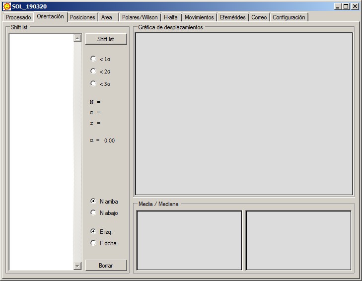
Once Iris has aligned the sequence of images, in the Orientation tab, on the left appears the content of the file (where each entry is preceded by the number of the image within the series) and simultaneously, a linear fit is made and the angle that we have to rotate the image is calculated so that the solar north is up.
Likewise, the graph shows the center of the solar disk in the entire sequence of images. The blue dots indicate those whose difference with the fit is less than the standard deviation (e <s); those of orange color are points whose difference with the adjustment is between the standard deviation and the double of said value (s <e <2s); and those of red color, those whose difference is more than double the standard deviation (e> 2s). The line is the result of the least-squares adjustment.
The scale of the axes is automatically adjusted to each case. This may assume that if the angle between the E-W direction and the X-axis is high, the apparent scatter in the graph may appear smaller than with a low angle. Therefore, to verify the reliability of the data, we should not be guided by the graph, but by the values of sigma and the correlation coefficient.
Initially all values are included in the calculation. However, in anticipation that some of the images have been misaligned, we can discard the most discrepant values depending on the standard deviation. Under the "Shift.lst" button we have:
<1 .- Only those values whose difference with the adjustment is less than the standard deviation are considered.
<2 .- Only those values whose difference with the adjustment is less than double the standard deviation are considered.
<3 .- Only those values whose difference with the adjustment is less than three times the standard deviation are considered.
Generally, a value of 2s usually goes well in most cases.
In addition, the following data appear:
N.- Number of data considered.
Sigma.- Standard deviation.
r.- Correlation coefficient.
Alpha.- Angle that we have to rotate the image so that the solar north is above. This angle includes 2 corrections: the deviation of the camera from the direction E-W, and the angle P.
Although the program automatically performs all the above, it is also possible to do it with the "Shift.lst" button provided that the file is in the working folder.
It is considered by default, that in the original sequence of images, the North is at the top and the East at the left, that is, the Sun travels the field from left to right. However, it may happen that, due to the optical configuration or the orientation of the camera, this is not the case, so that we may have to invert the image vertically or horizontally. In the lower part we can mark in what case we are.
Finally, with the "Delete" button we can delete the content of the windows, which allows us to process several sequences of images without having to restart the program on each occasion.
Below the main graph there are two other graphs with the variations of the mean intensity and the median along the whole series. In an ideal series, both graphs would show a horizontal line. However, vignetting makes the values at the ends somewhat lower, and on the other hand, changes in transparency, mainly due to the passage of clouds, produce irregular variations as well as a central peak more pronounced in the median. In parentheses, the range of both is indicated. In general, worse conditions imply higher values of the range.
Positions
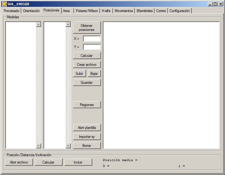
This tab is used to measure the positions once the oriented image has been obtained.
In this image, a spot is chosen, it is boxed, and when we click on the "Get positions" button, SOL will obtain the coordinates of the photometric center and automatically calculate the heliographic coordinates.
You can also manually enter the coordinates (x, y) of the spots, in the corresponding boxes, and with the "Calculate" button you can obtain the heliographic coordinates.
Next, each position must be assigned to a spot. To do this, in the second window, the NOAA group number is manually entered, followed by one, two or three letters that identify each spot. (At the end, the criterion used is explained).
The number of characters that the program supports is 5 digits for the region and between zero and three letters for the group and the spot. If the region does not yet have identification, it is possible to enter only the letters, or leave the entry empty.
To help in the identification of the spots, with the button "Regions" a window is opened where an image of the SOHO annotated will be downloaded (whenever it is available). In the window we can select the day (as of October 1, 2001) and the resolution of the image. Before January 14, 2011, the only resolution available is 512.
In case the SOHO image is not available, alternatively, the Solarmonitor button allows you to download an image in white light from www.solarmonitor.org. It should be noted that by default, we will always try to download the SOHO image first, each time we open the window or change the date.
Once we have finished, with the "Create file" button the measurements appear in the window on the right with the format used in Parhelio. The rotation number and the corresponding ephemeris are added in the lower part. The Up / Down buttons allow reordering the different entries in the final file, and the "Save" button saves a text file with the contents of that window.
With the "Delete" button we eliminate the contents of the windows, which allows us to process several sequences of images without having to restart the program on each occasion.
Every time we calculate a position, the coordinates (X, Y) of the spot are written in a file called "xy.txt", in the working folder. The program does not use this file, but it contains all the necessary data to calculate the positions and it is useful if later we want to reprocess the image or identify any possible error in the measurements. The "Import xy" button reads this file and displays the positions in the left window.
If we want to measure an old image, we can do it in two ways:
- The image (k2.fit) and the file xy.txt are placed in the working folder. With "Import xy" the measurements are loaded. Once the image is open, we can obtain more measurements that will be added to those we had already made. In this way we obtain a file where the old measurements are combined with the new ones.
- The image (k2.fit) and the corresponding sol.lst file are placed in the working folder. Then we enter the day and time of the image in the Traitment tab, and click on "Open template" to load the values of the file in the internal variables of the program. From that moment we can open the image and make the measurements. In this case, the file is created from scratch and only contains the new data.
In the lower part, we can do some additional calculations in groups of bipolar spots.
If in the right window we select two spots and click on the "Calculate" button, the program obtains the average position, the distance between both, in degrees and km, as well as the inclination with respect to the equator of the line that joins them.
The calculations are made along the maximum circle that passes through both spots. The inclination i, is considered positive if the latitude of the spot f is greater than that of the spot p, and negative in the opposite case.
With the button "Open file" we can load in the window a file of measurements previously created by Sol, or with the same format, to perform those operations on it. The "Include" button adds these calculations to the final file.
Areas
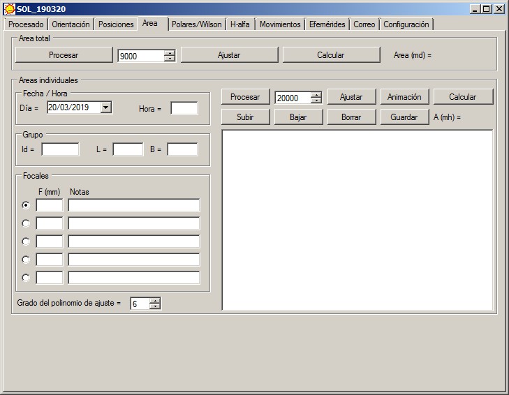
The window is divided into two parts that allow measuring the total area covered by the spots, or the individual area of a group or a spot. The theoretical aspects of the method to calculate them are explained on the following page: http://www.parhelio.com/docareas.html
It is not advisable to measure areas of individual groups on images of the whole disk, because errors can be important.
The measurement of the total area can be used as an activity index, especially if the data of several observers are combined and monthly averages are obtained.
In the upper part of the window you can calculate the total area covered by the spots, from an image of the entire disk. For this, it is necessary that in the working folder the image without limb darkening (k3.fit) is found, and the file with the parameters of the template associated with that image (sol.lst).
With the "Process" button, the program performs a series of operations whose result is an image with a white background and black spots. These spots coincide with sunspots, although other spots (usually simple black spots) due to granulation and a certain noise component may also appear. If the value in the box is too high, the black areas can cover a large part of the disk.
The way of operating depends on how the image is:
- If both types of spots appear, we decrease the value of the box one step, and the "Adjust" button recalculates the image. We will notice that the points due to the granulation decrease. You have to reduce this value step by step until only sunspots remain. It is important to make sure that all the pixels associated with the granulation disappear. At that moment, with the "Calculate" button we obtain the area.
- If only the sunspots appear, we increase the value of the box until the granulation appears. Then we reduce it one step and calculate the area.
For example, we go up (10000-10500-11000-11500-12000), and when we reach 12000, the granulation starts. So, the value that serves us is 11500.
In the box, the value is modified in steps of 500, but if you write it manually, you can put any other value and adjust it more precisely; although normally, this is not necessary.
The total area is calculated in millionths of disk (md), unlike the area of individual groups, which is obtained in millionths of hemisphere (mh); and therefore, they are not comparable.
To obtain individual areas, proceed as follows.
It is important that the image is cropped. It is necessary to leave out any sector of the limb and areas close to it, since otherwise, the background will not be well calculated. On the other hand, it is convenient that in the image only the zone of the photosphere closest to the group appears (although it is not good to adjust too much), to avoid residual gradients.
To trim, in Iris, a rectangle with the mouse is selected around the group. Clicking with the right button, you choose "Crop" ("Fenêtre").
SOL will calculate the area in the image that is on the screen when the process starts. The image should be black and white and preferably without having undergone previous treatments.
First of all it is necessary to enter the day and hour to which the photo is made, the denomination of the group (NOAA numbering), and its longitude and average latitude. If in the Positions tab we have calculated the average positions and have included them in the final file, the position will appear automatically when writing the number of the region.
On the left you can enter 5 different focal lenghts that are automatically saved among the preferences. That way, if one day we use a different optical configuration, we will only have to choose the one that corresponds.
With the Process button, the gradients are eliminated and the histogram is adjusted to increase the contrast.
In the box to the right, we must indicate the approximate intensity that corresponds to the edge of the penumbra. A simple way to determine it is to pass the cursor through the areas free of spots. In the lower right corner of Iris we will see the intensity values. The edge of the penumbra has a somewhat lower intensity than the photosphere; around 95%. At first, a lot of precision is not necessary, since we will make the necessary corrections later on.
With the Adjust button, the program will create an image in which all the pixels with less intensity than indicated will appear black, and if their intensity is greater they will appear white. By modifying the intensity we must look for the best fit between the black spots and the edge of the penumbra.
The Animation button will help us to check the goodness of the adjustment, overlapping at intervals the mask to the image.
Once satisfied, with the Calculate button we will obtain the area in millionths of hemisphere, and an entry will be added to the lower window.
With the buttons Up, Down, and Delete, we can sort the list or delete entries. Finally, we save a text file with the contents of the window.
Occasionally, especially in the case of very large and dark spots, it is possible that the Process button will introduce additional gradients. Sometimes it is possible to solve the problem by reducing the degree of the background polynomial fit. You can check its effect by modifying its value in the box under the focal points, opening the cropped image, and using the Process button again.
Polar/Wilson
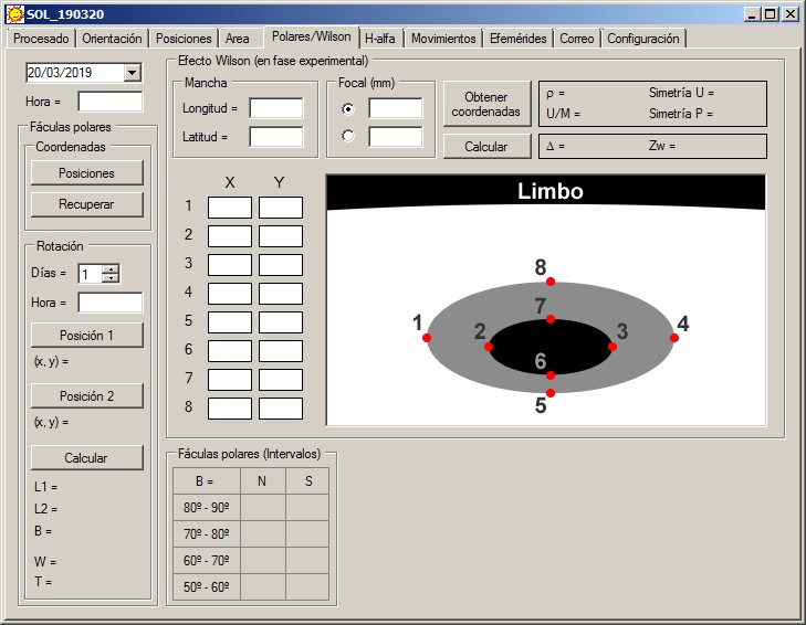
This tab includes two sections: polar faculae and Wilson effect.
Polar faculae.-
From the images in polar coordinates, the program allows to determine the heliographic coordinates of the polar faculae. Being close to the limb, the accuracy of the measurements in general is less than that achieved with the spots. On the other hand, the number of faculae is usually higher than that of spots.
For these reasons, SOL uses a less precise method, but faster. If the same method were used as with the spots (determining the photometric center), too much time would be spent without appreciable improvement in errors. In addition, in principle our objective is to obtain the total number of faculae and latitude intervals, as well as to represent a latitude-time diagram that shows its behavior over time, for which a very high precision is not required.
Once the image with both poles is opened in Iris, the Output window is deleted and it is verified that the date and time of the image appear in the Polar / Wilson tab. Then, with the mouse, we click on all the faculae, and in the output window the coordinates (x, y) of the chosen pixels and their intensities appear. Once we have finished, in SOL click on the Positions button and in the work folder there will be two files; one with the coordinates in the image (xypolares.txt), and another with the heliographic coordinates of each facula (aammdd polar OBS.txt).
From the first file it is possible to obtain later the heliographic coordinates with the button Recover; always taking care that the date and time are correct.
Likewise, the number of faculae in each latitude interval appears in the lower table of the window. The table also offers, as information, the latitude of the center of the disk, which gives an idea of the visibility conditions of each cap.
This part of the program also allows calculation of rotation periods using polar faculae. This aspect is of interest because the periods of rotation in high latitudes have been less studied than in the areas where the spots appear.
The main difficulty lies in the duration of the faculae, which rarely exceed one or two days, and in correctly identifying them on successive days. Therefore, only good images should be used and provided they have been obtained on consecutive days. If one day we have not observed, it is better not to use the images of the previous and subsequent days, because it would be difficult to assure which faculae have been maintained during that interval.
In this case we need all the possible precision, so the method is similar to the one we use with the spots.
Once a facula has been identified that has lasted more than one day, the date and time of the first image is entered into the program. In the section Rotation, the difference in days between the first and the last image is introduced (without taking into account the time). This default value is 1. Below is the time of the last image.
In the first image, the facula is boxed with the mouse and with the "Position 1" button the coordinates (x, y) of the brightest pixel are captured. The same is repeated with the last image and the "Position 2" button.
In the lower part, the initial and final heliographic lengths (L1 and L2), the medium latitude (B), the angular velocity (W) and the rotation period (T) appear. Although the calculation is done automatically when entering the second position, these quantities can also be obtained with the "Calculate" button.
Wilson Effect.-
(Important: This section is in experimental phase)
For the measurement of the Wilson effect it is necessary to have images with a good resolution and therefore, with a high focal. The images of the whole disc are inadvisable. It is for this reason that this section has a series of restrictions that avoid very high errors. The program will first check the uncertainty in the measurement and only show the result if certain values are not exceeded.
First of all, you must enter in the Polar / Wilson tab, the date and time of the image, the longitude and latitude of the spot, and the focal. The program can save a pair of focal lenghts so that we only have to mark the one we are using. As it happens in other sections, it is essential to previously obtain the effective focal lenght to which we are working, since the one indicated by the specifications of the instruments is not always correct.
In Iris we open the image of the spot and after deleting the Output window, we click with the mouse in eight points of the image. SOL includes a scheme where it is indicated which points it is and the order in which it is necessary to mark them; the first four following a direction parallel to the limb, and the other four in a perpendicular direction, and in the direction center -> limb.
The Get Coordinates button will extract the coordinates (x, y) of each point from the output window. These values will be included in the boxes to the left of the diagram, although they can also be entered manually. With the Calculate button the following quantities are obtained:
r.- The heliocentric angle between the spot and the center of the disc.
Symmetry U and P. - These values indicate the degree of symmetry of the umbra and the penumbra. A value of 1 indicates a circular umbra or penumbra. It is not advisable to obtain the Wilson effect in asymmetric spots.
U / M.- Quotient between the diameters of the umbra and the penumbra. It allows to check variations in its relative size depending on the greater or less distance to the limbus.
D.- Wilson Effect. If the spot has this effect, D> 0, if it does not, D = 0, and if it is inverse, D <0.
Zw.- The value of Wilson's depression, that is, the depth in km from which the radiation of the umbra seems to come.
H-alpha
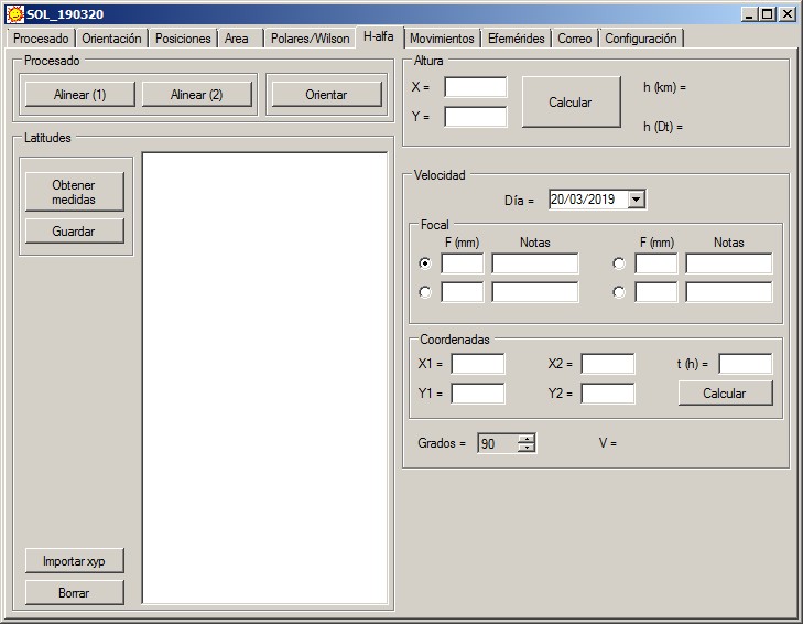
This tab allows to perform various geometric calculations on the prominences.
With H-alpha images the processing is similar to the images in white light, using the two buttons at the top, although it has the following differences:
1.- The Raw -> Fit conversion is done in color, so before aligning the images the program will separate the 3 channels and eliminate the G and B channels. This step may take a few minutes.
2.- The disk and the limb are processed separately; the first one as the images in white light, and the second, masking the disk.
In this section you can also use the two methods of alignment that we saw in white light.
At the end of the H-alpha process, an image of the limb that can be used to obtain latitudes and heights is shown. The section "Speeds" is intended to be used with animations, or at least, with images that have been obtained with the same optical configuration, with the same dimensions and orientation, and that have been previously aligned.
It is assumed by default that a video camera whose pixels have the dimension specified in the Configuration tab, Areas section, is used for the calculation of speeds.
Latitudes.-
A prominence is an extensive structure that generally encompasses a more or less large sector of the limb. In Iris, we will use the cursor to determine the coordinates (X, Y) of the ends of said sector, and the program will calculate the average latitude, the position angle (measured from the N, in the NESW sense), and the extension of the prominence in heliographic degrees. These values are added to the window, and can then be saved in a text file.
The method consists of taking advantage of the data that appear in the Output window of Iris. Each time we click on the image, three data appear in the window: the coordinates of the pixel where we clicked, and its intensity. The method consists in marking one after the other, with the mouse, the north and south ends of each prominence.
When we have finished, we will use the "Get measurements" button. In this way, the program reads the contents of the output window, and automatically calculates the latitudes and extensions of the protuberances.
The program will automatically create a file called "xyp.txt", with the necessary data to carry out the calculations later if necessary. The "Import xyp" button allows you to perform this operation.
Heights.-
In the same way as in the previous case, we can obtain in Iris the coordinates (X, Y) of the highest point of the protuberance. These coordinates can be entered in SOL and obtain the height above the surface, in km and terrestrial diameters.
Speeds.-
The ideal to determine speeds, is to take advantage of a sequence of images designed to produce an animation of a protuberance. The images, therefore, have to meet the conditions mentioned above: the optical configuration, dimensions and orientation must be the same; and it is necessary that they have been aligned with the limb as a reference.
As in the calculation of areas, the program keeps several focal lenghts so that we only have to mark the one we used in the observation. The date, the focal length and the size of the pixels (in the Configuration tab), are the data that allow us to determine the scale of the image and transform pixels in km.
With Iris the position of a detail in two of the images is measured, and the coordinates (X1, Y1), (X2, Y2), we will introduce them in the program together with the interval of time elapsed between both images (in hours).
Since we do not know the angle between the direction of movement and the visual, we can not know what the real speed is, but at least we can limit it. If we assume that the displacement is perpendicular to the visual, the obtained value is a minimum speed.
When we click on the Calculate button, the program determines the speed assuming that the displacement and the visual are perpendicular. However, we have the option to vary the angle between 5º and 90º and obtain the speed in each case. Logically, for an angle of 0º the speed would be infinite.
Motions
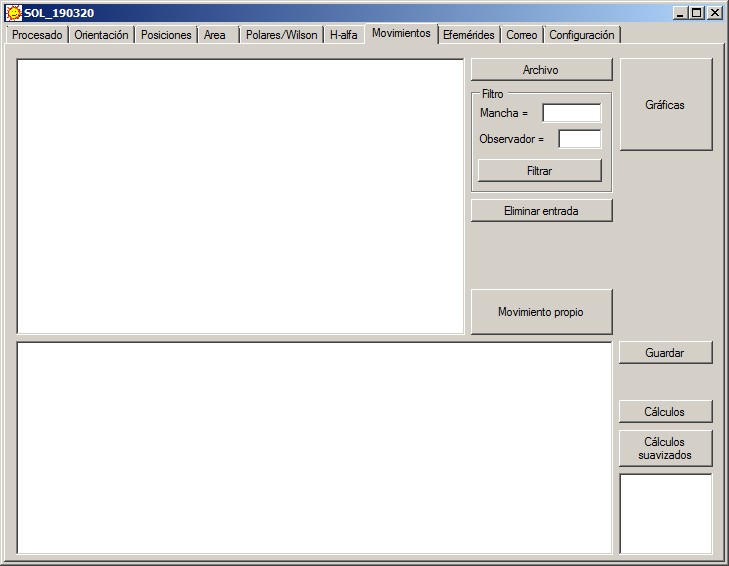
The "Motions" tab allows you to calculate the movement of a spot from its position measurements. This section analyzes the measurements of a single observer, and is not intended to combine measures of several observers. However, if the positions of several observers are previously averaged, the resulting list can be used as a starting point to obtain the proper movement with SOL.
In principle, it is necessary to have a text file that includes all the measures of the spot, such as those found in http://www.parhelio.com/en/posic.html We can also create it by copying and pasting in a text file all the measures that we have made of a spot, or those we made during the transit of the spot or during a rotation, for example. The only condition is to keep the format used by SOL.
The File button opens the text file with the measurements, and we can filter the entries by spot name and by observer code. In case any measure is very discrepant or contains an error, it can be eliminated using the Delete entry button.
Once we have the positions corresponding to a single spot and a single observer, we perform the calculations using the proper motion button. The result appears in the lower window.
The columns correspond to the date, time, longitude and latitude. DLong and DLat are the proper motion in longitude and latitude, taking as origin the first measurement. These amounts are calculated as explained in http://www.parhelio.com/en/mp.php
DLongS and DLatS correspond to the smoothed path, calculated by means of a moving average, averaging 3 consecutive measurements.
"Proper motion" also makes the following amounts appear in the small window, located on the bottom right:
N.- Number of days between the first and last position.
D.- Distance in degrees traveled along the trajectory.
V.- Average speed calculated along the trajectory.
W.- Angular speed.
T.- Period of rotation.
If we select two different dates in the left window, the Calculations button determines those quantities between the new dates. Smoothed calculations do the same, but with the positions of the smoothed path.
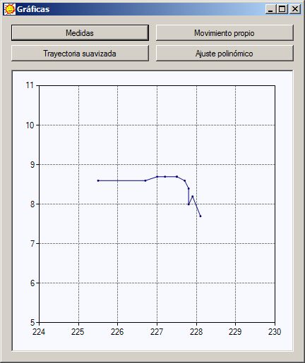
The Graphs button opens a new window where we can represent the measured positions, the proper motion, the smoothed trajectory, and an adjustment by means of a third degree polynomial. These buttons will only work if we have previously calculated the proper motion and we have a minimum of 3 measurements.
The positions of the polynomial fit correspond to the 12h UT of every day between the first and last measure. This type of adjustment must be considered with certain reservations, especially at the ends of the trajectory where its error is greater.
Each time we create a graph, the program copies it to the clipboard, so if we want to export it, we just have to open another application and do Crtl + V or "Paste".
Ephemeris
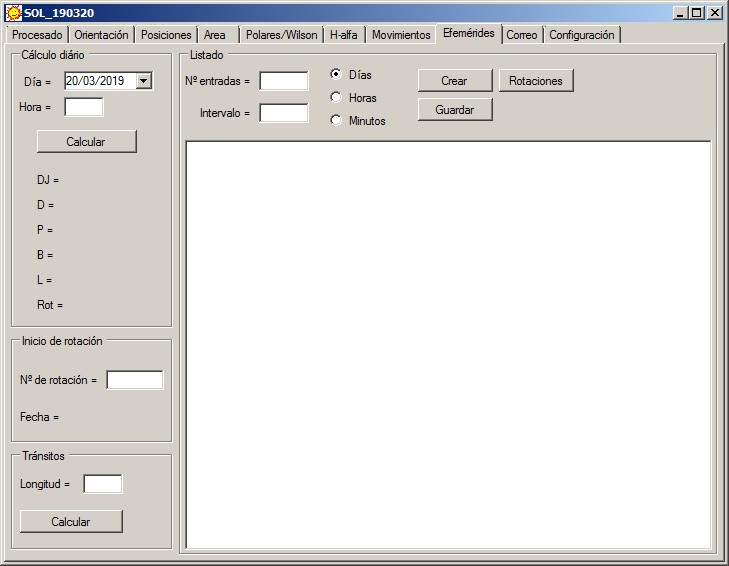
This tab allows the calculation of ephemeris independently of the rest of the functions.
Once the day and time have been entered, the "Calculate" button shows the ephemeris for that moment:
DJ.- Julian Day
D.- Solar diameter in seconds of arc.
P.- Inclination of the axis of solar rotation, with respect to the N-S direction.
B.- Heliographic latitude of the center of the solar disk.
L.- Heliographic length of the central meridian.
Rot.- Number of rotation.
In the lower part, if we enter the number of a rotation, we obtain the start date of it.
The controls on the right allow you to obtain listings with a certain number of entries. "Interval" is the difference in days, hours, or minutes, between two consecutive entries. With the "Create" button we obtain the data.
The list consists of 6 columns: Date, time, P B, L and rotation. If the rotation number is negative, it will not appear in the list.
With the button "Rotations" we calculate the date and time of beginning of as many rotations as we indicate in the "Nº of entries", obtained from the rotation introduced below on the left.
The section Transits serves to determine the dates in which a certain heliographic length passes through the visible hemisphere. In the upper part of the window it is necessary to enter a departure date and the number of entries (transits) that we want to obtain.
When we put a length in the corresponding box and click on the Calculate button, the dates appear in which said length coincides with the limbs E and W (start and end of transit), and its passage through the central meridian.
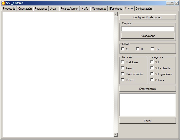
Once we have finished obtaining measurements and images, the program allows its sending by mail.
First of all, click on the "Mail Settings" button. In the window that opens we can configure the account as in any mail client. The program supports three possible destination addresses.
In the Folder box we have to indicate the address of the folder where the measurement and image files are located.
In Data, we have the option to include some entries in the body of the message to write the number of groups (G), the number of Wolf (R), or the visible spots with the naked eye (SV).
Below we indicate the files (Measurements and Images) that we want to include as attachments. When clicking on Create message, in the bottom window the files that you have found in the folder are indicated, and on the left, what will appear in the body of the message. We can freely modify your content before sending it.
Measurement of positions step by step
- Iris.- The images are converted to fit b & n format, with the menu "Digital photo" ("Photo numeric"), "Decode RAW files ..." ("Décodage des fichiers RAW ...").
- SOL.- Enter Day / Time, generic name and use the Align (1), Align (2) button, or manual alignment.
- SOL.- In the Orientation tab we obtain the angle alpha.
- SOL.- Orient button to finish preparing the image.
- Iris / SOL.- The position of a spot is calculated by selecting it in a box. Then, with the button Get positions we calculate the heliographic coordinates.
- Iris / SOL.- Repeat the last two steps with all the spots.
- SOL.- In the second window the identification of each spot is written.
- SOL.- With the button Create file, we put the measurements with the appropriate format.
- SOL.- We save the result with the Save button.
What to measure
When we are ready to measure the positions before an image of the Sun, the first question we ask ourselves is "What spots to measure?".
Perhaps the best advice that could be given is to resist the temptation to measure everything. It is necessary to take into account that it is not a question of mapping the group, because for that we already have the images, but to obtain a series of parameters such as the proper motions, periods of rotation, linear and angular speeds, inclination of the group axis, etc ...
This is only achieved by choosing those spots that can offer a greater number of measurements, that is, those that measure the greatest number of observers during the greatest number of days. This is why it is better to measure larger spots, because they will probably last longer.
It is no good measuring small spots that are next to a large one, because most likely we only get that measure, and by measuring the main spot we already get all the necessary information.
The same can be said of the central spots of a bipolar group, although they have a certain size. Only exceptionally, when they have a peculiar behavior, it is worth measuring them.
Of course, most of the time it is difficult to guess a priori, the evolution of the spots. However, if we keep the image k2.fit, the template sol.lst and the file xy.txt, the program has the necessary tools to make additional measurements on images from previous days (see section "Positions")
In addition, measuring many spots is often counterproductive because it makes us lose a fundamental data when combining the measurements of an observer with the rest. If in a group with many spots we obtain only one or two positions, we know for sure that they will correspond to the darkest spots. On the contrary, if we measure, for example, 10 spots, we will not know which of them will be the darkest, and therefore, which will be the ones that have been measured by the rest of the observers.
Given the enormous variety that groups of spots can present, it is complicated to establish very precise rules, but general rules can be followed:
- If the group is unipolar (morphologically speaking), we will obtain only one measure, usually from the main spot. It is best to select the largest spot, or select the whole group and let the program choose the darkest spot.
- If the group is bipolar, we will obtain only two measurements on the spots p and f. It is best to select the entire p region and let the program measure over the darkest spot; and then, repeat the process with the region f.
In case of complex groups, the list of positions on the page (http://www.parhelio.com/en/posic.html) can be used as a guide, where we can check which are the spots that accumulate a greater number of measurements.
About the nomenclature
First of all, it is necessary to distinguish the concepts region, group and emersion. In the absence of a precise definition of "group", there may be some confusion or ambiguity, and the three concepts are not always going to be perfectly delimited.
An active region is the area of the surface where the groups of spots appear (although it also manifests itself in the chromosphere and the corona). NOAA numbering refers to active regions.
The magnetic field that forms the spots, does not come to the surface continuously but in impulses. We call each of these impulses "emersion". Depending on where and when an emersion occurs, it can be considered an independent group or not.
For example, if in the same active region two emersions take place at several degrees of distance, we will normally consider them as two groups. Now, if an emersion occurs in the center of an already established group, we would continue to consider it a group.
The nomenclature we use uses the NOAA numbering followed by letters that allow us to identify the groups and spots according to their situation. The correct way to read it is:
Region - Secondary group - Main spot - Secondary spot
Depending on the case, all terms can be used or only some.
The letters used are: p and f for the main spots of a group, and n, s, e, w for the groups or secondary spots. Any letter in front of p or f always refers to a group, and if it is behind, it will indicate a spot.
Let's see some examples:
If in a region there is only one spot, it will suffice to indicate the number of the region (the evolution of the group will impose an exception to this rule that we will see later).
If in a region there are 2 groups, the main one (or the first one that appears through limbo) will receive only the number of the region; and to the secondary we will add a letter depending on your situation with respect to the main one:
12004n.- Secondary group located north of the main one in the region 12004
12014p.- Spot p of the main group of 12014
12014np.- Spot p of a group located north of the main one in 12014
12021pn.- Secondary spot located north of spot p of the main group in 12021
11974efn.- Secondary spot located north of spot f of 11974e.
Important.- Note that the order of the letters is fundamental. It is not the same 12014pn as 12014np. Both denominations would refer to different groups: the first case would refer to the main group of 12014, and the second, to a secondary group located north of the main group.
To avoid confusion, especially when analyzing the measures, it is advisable not to change the denomination of the spots throughout the life of the group. For example, group 11987 started being bipolar so we measured spots 11987p and 11987f. However, after days disappeared all except p. With this spot it is advisable to keep the denomination 11987p, despite being the only one that remained in the active region.
This way of naming the spots is not without ambiguity. For example, if in region 11989 the main group consists of only one spot; 11989s can refer to a secondary spot belonging to 11989, or to an independent group located south of the main one. However, if we follow the general rules outlined above, and avoid measuring secondary spots, this case will not occur almost never.