Latitude

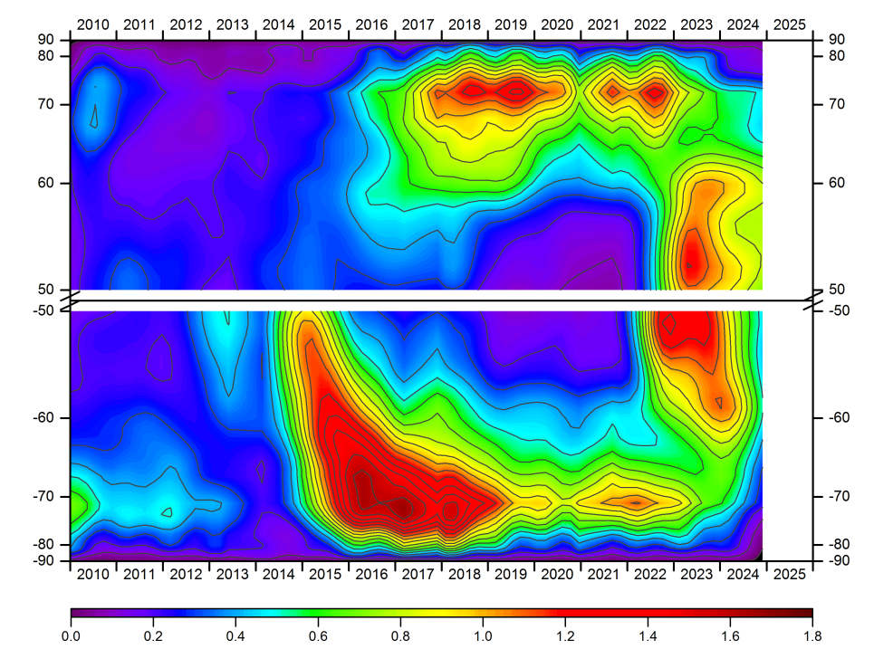
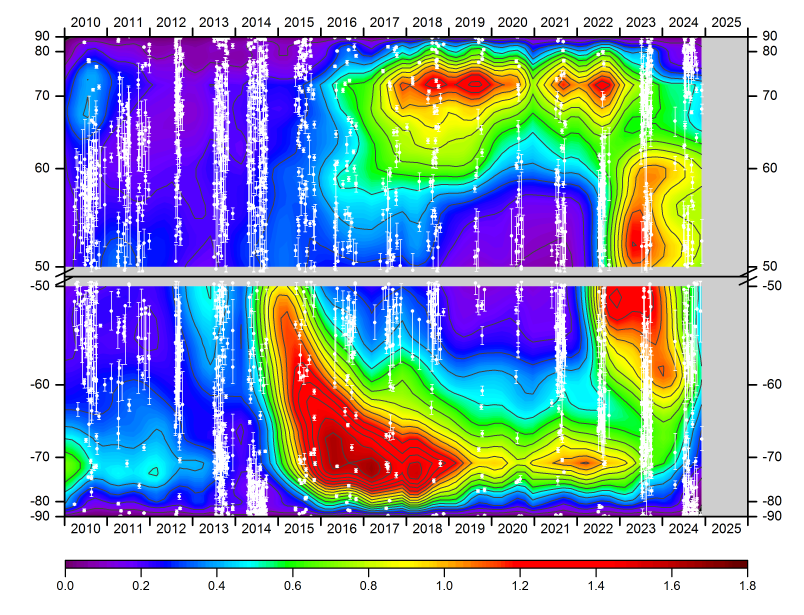
The following graph is a diagram similar to that of Maunder, or latitude-time diagram as the one that is elaborated for spots or prominences, but in this case for polar faculae. It represents the latitude of more than 50000 faculae recorded since 2010, in both hemispheres. On the Y axis the latitude sinus is actually represented. This is useful because in a sphere, the relationship between the surface of two latitude intervals is the same as the lengths of those two intervals in the graph and, therefore, it is the most suitable representation to visualize the relative densities between different latitudes. .

The method to carry out the measurements can be consulted at http://www.parhelio.com/en/docpolar.html

Position data can be found in http://www.parhelio.com/en/faculasdatos.html

To improve visualization and highlight the most relevant features, densities have been calculated, smoothing the data and applying contour lines. The values of the scale represent the monthly average of facula per degree of latitude:

In the following links there are also some animations that show how the density of faculae varies according to the latitude over time. The interval between frames is 100 days:

www.parhelio.com/faculas/animn.avi
www.parhelio.com/faculas/anims.avi

When interpreting these graphs it is necessary to consider some aspects:

- During 2010, a 100 mm f /10 refractor was used with a Nikon D40. Since the beginning of 2011 the telescope is a refractor of 120mm f /7.5, and since the end of 2013 the camera is a Nikon D3200. It does not seem that both changes have had much effect. However, as the current instruments offer images of higher quality and resolution, we can not rule out the existence of a certain "bias" in the number of faculae compared to the first years.

- Every year, from November to February the telescope is in a different location, where the images are of lower quality. In those months, the number of images used is usually lower, which causes gaps in the graph and a certain annual modulation by registering a greater number of faculae in the summer months than in winter. When the same trait is repeated in both hemispheres, it is mainly due to this cause.

- As with other indexes, faculae counts depend not only on the image quality, but on the observer's criteria when deciding what is or is not a facula. This factor makes more or less points appear on the graph, but does not alter the areas of higher density.

- The inclination of the axis of solar rotation means that the south pole is observed in better conditions in February-March-April, and the north pole in August-September-October. This circumstance originates an annual variation in the graph, where a sinusoidal envelope appears above 75º of latitude.

- The minimum of activity has meant that fewer photographs have been taken and that the follow-up is more deficient in 2018.

Until 2014, the faculae are concentrated in latitudes greater than 70º in both hemispheres. However, in the north they tend to move towards the pole while their number decreases. In the south they remain without many changes until 2012 and then reproduce the same process that had the north during the first years. The most interesting behavior took place in the south as of 2014. That year, the faculae start to increase between 50º and 60º, and in 2015 the activity extends throughout the cap. From that moment a migration towards the pole takes place, reducing more and more the range of latitudes in which they appear.

In the north, the situation is more confusing, perhaps due to the evolution of the magnetic field in that polar cap, which remained with a low intensity during the years 2012-2013-2014, presenting up to three inversions of polarity in that period. Only in 2017-2018 the density of faculae has been comparable to that of the south.

Another way to visualize these changes is to represent the positions (longitude, latitude) in polar coordinates for each year and hemisphere (north up and south down). Clicking on the graphics gives access to higher resolution versions.

Link prominences - faculae

Both the number of polar faculae and the latitude of the protuberances provide information about the caps and it is not surprising that both phenomena are related to each other. The faculae are formed inside the caps and the protuberances at their edges, so that both will not coexist in the same regions. In addition, the reduction in the size of the caps throughout the cycle will cause the migration towards the poles, both facula and protuberances. In the following graphs we have superimposed the latitude-time diagram of protuberances (see here) to that of faculae.

We have the clearest behavior in the south. Between 2012 and 2014 the drift of the protuberances occurs, precisely occupying the corridor left by the faculae. Once the former have reached the pole, faculae begin to form in ever greater latitudes. In the last years of the cycle, the protuberances are kept at about 55 °, while the regions closest to the pole are occupied by the faculae.

In the north, the situation is more confusing, although it can also be seen how migration of protuberances as of 2010 occurs along the faculae-free latitudes. The low magnetic intensity between 2012 and 2014 is reflected in an abundance of protuberances and shortage of faculae. Only as of 2015, the number of protuberances decreases and the number of faculae begins to increase.

Total number of faculae

The first graph shows the monthly average of faculae and their softened values in the north and south polar caps, at a latitude greater than 50º. The second represents the daily averages throughout the Sun, without separating by hemispheres, and provides us with a global perspective. Although counts can be made directly on the images, the data in the following graphs have been extracted from the position measurements represented in the previous sections.

On the left you can see the annual oscillation produced by the inclination of the axis of rotation. The activity in the south has been systematically greater than in the north until 2018, at which time both hemispheres have balanced. On the other hand, it should be mentioned that the faculae do not disappear at all, even during the maximum cycle.

Number of faculae by latitude sectors

To analyze the variation of the latitude, each cap has been divided into four intervals of 10º each, between 50º and 90º of latitude, and counts have been made separately in each one of them. The following graphs represent the monthly averages for each cap and each latitude interval.

As expected, the annual variation is predominant above 70º. To give an example, the parallel at 70º of latitude covers about 140º of longitude in March and about 220º in September, that is, a difference of 80º throughout the year, while with the parallel at 50º, that difference is reduced to less than 20º. In fact, in the fourth interval, above 80º, counts can not be made during several months of the year.

Perhaps the most outstanding behavior is that of the southern hemisphere. In 2014 there was a sudden increase in activity below 60º, and at the beginning of 2015, the activity outbreak occurred in the second interval (60º-70º). At the end of that year, the increase in activity reaches the latitudes above 70º, while in the first interval it decreases until reaching almost the levels prior to 2014. What the graphs are revealing is a migration of faculae from latitudes around 55º to the pole, just after the maximum of the cycle. If we superimpose the graphs of the first three intervals, it can be clearly seen that over a year and a half, the increase in activity occurs in ever greater latitudes:

With the previous counts you can also make a diagram similar to the one presented at the beginning, although in this case the resolution is quite low since the data are monthly values and we only have four latitude intervals.

In it you can see both the annual oscillation above 70 °, as migration in the south from 2014. It is also worth mentioning that the gap between hemispheres showing the activity of the sunspots, was reversed in mid-2015, so that since then, the south is ahead of the north. However, the polar faculae show that advance about a year before.