Next, we describe the method we use in Parhelio, both to measure the total area (in millionths of disk), as well as the areas of individual groups (in millionths of hemisphere). The difference between both is that the individual areas are corrected by perspective, but not the total areas, since it is very complicated to make this correction on images of the entire disk.

To obtain the total area in millionths of the hemisphere, the individual areas are added.

The programs used are Iris and SOL. Their joint management is explained in the section on Position Measures, and in the documentation of SOL.

Here we will describe the most theoretical aspects, although SOL performs all this treatment almost automatically, as can be seen in the previous links.

A comparison of the results can be seen in the article "Comparación de las medidas de área de Parhelio, de Debrecen y del SOON"

MEASURES OF THE TOTAL AREA

The measurements of the total area are made on the image that is used to measure positions. The preliminary process is described in Position Measures, and basically consists of capturing a sequence of images of the whole disk, without tracking, so that the diurnal movement of the Sun marks us the E-W direction.

SOL uses Iris to perform the processing of this sequence, aligning, adding, and orienting the resulting image. It is this image that we will use to measure the area.

However, first of all, it is necessary to suppress the limb darkening by means of the function "Eliminar gradiente" of SOL. The method used by this function is described in http://www.parhelio.com/doctecnicas.html

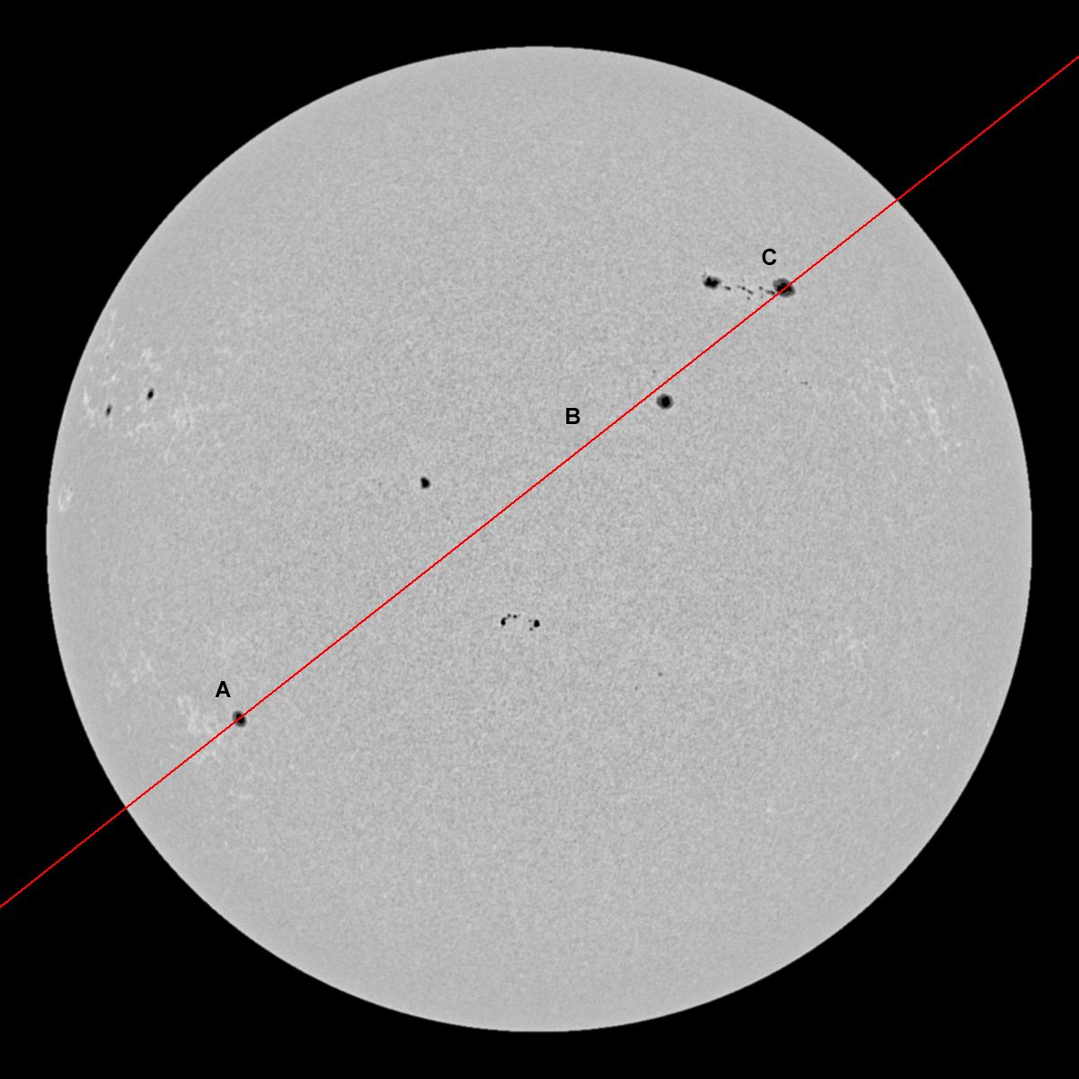
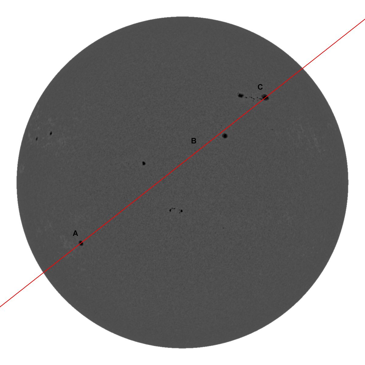
The result is an image whose sky background has a zero intensity, and the disk a constant average intensity. However, in the disc we find fluctuations that are due to 4 causes: spots and pores, faculae, granulation and noise. The spots and pores have a lower intensity than the average, and in the case of the faculae it is greater. On the other hand, granulation and noise have a random behavior around the mean value.

The next image has already gone through that process, and the graph shows the intensity along the red line. Two spots can be seen (A, C) and one pore (B).

The areas are calculated from that image. First, the program creates a synthetic image in which all the pixels that coincide with the solar disk have zero intensity, and those that match the sky background assign them the maximum intensity. Then add this image to the one we had from the Sun, and with this we get the skybackground to appear white while the disk does not change. The idea is to isolate the spots from the sky background.

In this image, the darker details are the spots and then, in order of increasing intensity we have the granulation and the noise, the faculae, and the sky background. Now it is easy to isolate the spots by defining a cutting intensity.

When we introduce an intensity in the program, it can assign the brightest pixels the maximum intensity, and the weakest ones a zero intensity. In this way, we can modify the value, in steps of 500, to facilitate our choice. Let's see some cases:

10000	9000	8500	8000

In the graph we have increased the vertical scale, marking 4 possible intensities.

Above 11500 the entire disc will appear black. Since the average disk intensity is 10,000 units, at that level approximately 50% of the pixels will be black. With 9000 there are still quite a few pixels associated with granulation. Looking at the graph, we could think that the good intensity is 8500. However, we must not forget that the graph corresponds to a line, not the entire disk, and when we introduce this intensity, we see that there are still some residual pixels near the center . Going down to 8000 and only the spots remain, so that will be the chosen value.

Next, the program determines the number of pixels that have less than 8000 counts, and since previously it had obtained the dimensions of the disk, the calculation of the area is immediate.

The total area can be used as an activity index, similar to Wolf number, although the information provided by both is different. Unlike Wolf number, the area is the measure of a physical magnitude, and the method employed minimizes the intervention of the observer. The differences between observers have their origin mainly in the following factors:

- The seeing, which worsens the definition of the edge of the penumbra and can make pores and smaller groups disappear.

- The characteristics of the image. Different values ​​of gamma, or of other parameters, can modify the position of the edge of the penumbra, and thus for example, less contrasted images usually provide larger areas.

- The resolution. At the edge of the penumbra, the area enclosed by an isofota contains fractions of pixels that generate an uncertainty in the count of the pixels. This error is inversely proportional to the size of the disk.

However, despite these differences, on a scale of days the area is more stable and has fewer fluctuations than Wolf's number. Using data from three observers during 2012, the relative error of the area with respect to the average was 7.3%. With the data of 12 observers, the error in Wolf's number in that period was 20.1%, that is, almost 3 times higher.

MEASURES OF INDIVIDUAL AREAS

The method to measure individual areas is similar to the one we have seen above, although in this case the type of images is different, the elimination of the gradient is done by another method, and we do not need to treat the sky background as it does not appear in the images .

Before performing the calculation, we need to know four things to introduce them into the program:

- Day and hour.
- The heliographic coordinates of the group, which we have previously obtained on an image of the entire disk. If the group is extensive, we will use the average position.
- The size of the pixels in micrometers.
- The focal lenght. It is essential to know it accurately and it would be advisable to measure it beforehand because there may be surprises, especially if we use a barlow. The focal lenghts used will be medium or high, preferably greater than 2m. It is not advisable to use the images of the whole disk, because a short focus contributes a lot of error to the measurements. In any case, it is not advisable to use too large focal lengths, because the edge of the penumbra would be poorly defined.

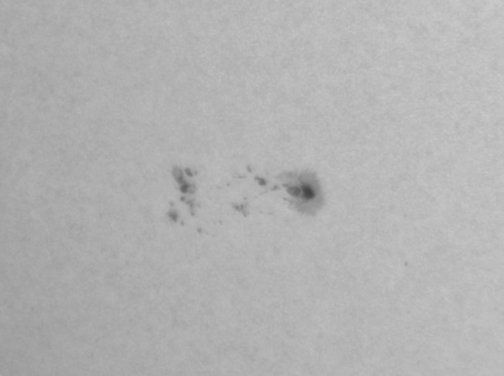
First of all, it is important to start with unprocessed images, and it is convenient to trim their edges. The first thing that the program will do is suppress the background gradients, but residual variations can always remain, and one way to reduce their presence is to reduce the field covered by the photo. However, it is not advisable to adjust the cut too much to the spots so that the process does not introduce artificial gradients. The important thing is that the intensity of the background of the image does not vary much, that is, if the spot is near the center of the disc, we may not need to cut, but it will be forced near the limb.

On the other hand, if the limb and the sky background appear in the image, we must cut them so that they are out of the image.

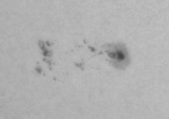
The program does a preliminary treatment, eliminating the limb darkening by means of the command >setsubsky of Iris, and adjusts the histogram to visualize the image with more contrast. It also performs a slight defocus to reduce noise and granulation. The objective of this operation is to better identify the intensity of the edge of the penumbra and ensure that the isofotas have a somewhat softer profile.

The method is similar to the one we saw before; The program assigns a zero intensity to all the pixels below a certain intensity, bringing the rest to the maximum intensity. In the example photo that we are using, with an intensity of 19000 no black pixels appear in areas of the photosphere, but the adjustment is not good, especially in the entrails of the penumbra. With 18500 the setting is more correct:

19500	19000	18500

Once obtained the intensity that we were looking for, the program obtains the pixels enclosed by the corresponding isophote. With the focal lenght and the size of the pixels, the scale of the image is calculated, the size of the solar disk are determined by the date and time, and with the position of the group we obtain the perspective correction. All this helps us calculate the area in millionths of the hemisphere.